2020 Syllabus and Course Mechanics

MAKE SURE TO READ THE SYLLABUS RIGHT AWAY IF YOU HAVEN'T!!!!!

YOU CAN GET FREE WALL STREET JOURNAL ACCESS THROUGH THE UNIVERSITY’S SUBSCRIPTION HERE!!! https://education.wsj.com/search/

Signing Up For Sapling

  1. Go to www.saplinglearning.com/login to create an account. If you already have a Macmillan Learning account you can log in with your existing credentials and skip to step 3.

    • Create your password and set all three security questions.

    • Start typing in your institution to select from the options that appears in the Primary Institution or School name field. If you institution does not appear you can add it by typing in the full name.

    • Accept the terms of use and click “Sign Up”.

    • Check your email for the confirmation link to complete your registration and return to the login page.

  2. Set your institution by searching using your institution’s full name and selecting the appropriate option from the menu that appears.

  3. Under Enroll in a new course, you should see Courses at [Your College]. Click to expand this list and see courses arranged by subject. Click on a subject to see the terms that courses are available.

  4. Click on the term to expand the menu further (note that Semester 1 refers to the first course in a sequence and not necessarily the first term of the school year).

  5. Once the menus are fully expanded, you’ll see a link to a specific course. If this is indeed the course you’d like to register for, click the link.

  6. To access your eBook click on the image of the cover on the right sidebar of your course site. Create an account or log in with an existing Macmillan Learning eBook account.

  7. Review the system requirements.

  8. Need Help? Answers to many common questions are found in our Student Support Community. If you need direct assistance you can also contact technical support:https://macmillan.force.com/macmillanlearning/s/.

If you find the above confusing, the following article might help:

https://macmillan.force.com/macmillanlearning/s/article/Sapling-Learning-Registering-for-courses

Course Evaluations Toward the End:

colorado.campuslabs.com/courseeval

2019 Final Exam

2019 Final Exam

Practice Final Exam

Readings:

2019 Syllabus and Additional Readings and Exercises

colorado.campuslabs.com/courseeval

YOU CAN GET FREE WALL STREET JOURNAL ACCESS THROUGH THE UNIVERSITY’S SUBSCRIPTION HERE!!! https://education.wsj.com/search/

Each of the supplementary reading assignments is listed under the textbook chapter or other heading most closely related to it. 

Course Mechanics: MAKE SURE TO READ THE SYLLABUS RIGHT AWAY IF YOU HAVEN'T!!!!!

  1. Go to www.saplinglearning.com/login to create an account. If you already have a Macmillan Learning account you can log in with your existing credentials and skip to step 3.

    • Create your password and set all three security questions.

    • Start typing in your institution to select from the options that appears in the Primary Institution or School name field. If you institution does not appear you can add it by typing in the full name.

    • Accept the terms of use and click “Sign Up”.

    • Check your email for the confirmation link to complete your registration and return to the login page.

  2. Set your institution by searching using your institution’s full name and selecting the appropriate option from the menu that appears.

  3. Under Enroll in a new course, you should see Courses at [Your College]. Click to expand this list and see courses arranged by subject. Click on a subject to see the terms that courses are available.

  4. Click on the term to expand the menu further (note that Semester 1 refers to the first course in a sequence and not necessarily the first term of the school year).

  5. Once the menus are fully expanded, you’ll see a link to a specific course. If this is indeed the course you’d like to register for, click the link.

  6. To access your eBook click on the image of the cover on the right sidebar of your course site. Create an account or log in with an existing Macmillan Learning eBook account.

  7. Review the system requirements.

  8. Need Help? Answers to many common questions are found in our Student Support Community. If you need direct assistance you can also contact technical support:https://macmillan.force.com/macmillanlearning/s/.

If you find the above confusing, the following article might help:

https://macmillan.force.com/macmillanlearning/s/article/Sapling-Learning-Registering-for-courses

Signing up for Sapling—which includes the textbook:

  • Go to www.saplinglearning.com/login to log in or create an account.

  • Under Enroll in a new course, you should see Courses at [Your College]. Click to expand this list and see courses arranged by subject. Click on a subject to see the terms that courses are available.

  • Click on the term to expand the menu further (note that Semester 1 refers to the first course in a sequence and not necessarily the first term of the school year).

  • Once the menus are fully expanded, you’ll see a link to a specific course. If this is indeed the course you’d like to register for, click the link.

  • To access your eBook click on the image of the cover on the right sidebar of your course site. Create an account or log in with an existing Macmillan Learning eBook account.

  • Need Help? Our technical support team can be reached by phone, chat, or by email via the Student Support Community. To contact support please open a service request by filling out the webform: https://macmillan.force.com/macmillanlearning/s/contactsupport.

  • The following link includes more detailed instructions on how to register for your course: https://macmillan.force.com/macmillanlearning/s/article/Sapling-Learning-Registering-for-courses.

On Writing and the Writing Assignments

On Reading and Learning

Chapter 1—The Science of Macroeconomics

Chapter 2—The Data of Macroeconomics

Chapter 3—National Income: Where It Comes From and Where It Goes

Chapter 4—The Monetary System: What It Is and How It Works

Chapter 5—Inflation: Its Causes, Effects and Social Costs

Chapter 6—The Open Economy

Chapter 7—Unemployment and the Labor Market

Chapter 8—Economic Growth I: Capital Accumulation and Population Growth

Chapter 9—Economic Growth II: Technology, Empirics and Policy

Chapter 10—Introduction to Economic Fluctuations

The Writing Assignments

Let me remind you of two important requirements for your writing assignment:

- Above the body of each post (but below the title), you need to write your thesis statement for your post

- One reference must be a 2019 Wall Street Journal article


I added these requirements to the instructions below. Please read them carefully.


1. You have to use Canvas (https://canvas.colorado.edu/) to turn in your writing assignment. In order to receive credits, you must submit your writing NOT ONLY to "Assignments" folder BUT ALSO to "Discussions" folder at the same time. Failure to submit your assignment to both folders would lead to no grade.


2. Your blog post in "Assignments" folder allows for automatic plagiarism check. Students who plagiarize will fail will get an failing grade. I will write a short comment on your writing. Your classmates can't see my comments on your writing.


3. Your blog post in "Discussions" folder helps your classmates read your writing. By clicking "Reply," you can write blog posts in "Discussions" folder. Please write comments on other blog posts written by your classmates.


4. For full credits, your blog posts must satisfy several requirements: 

- Between 400 and 600 words long

- Must link to at least 2 other sources. One of those two sources must be a 2019 Wall Street Journal article. The citation protocol in blogging is that you should have a functioning link AND enough information that the source can be googled if the link breaks

- Above the body of each post (but below the title), you need to write your thesis statement for your post

- Any writings that fail to meet these requirements can't receive full credits. 

Sample blog posts can be found at https://blog.supplysideliberal.com/intermediate-macro/2017/12/31/student-guest-posts-on-supplysideliberalcom


5. Your blog post will be due at 11pm on every Sunday. For example, the due date of your first assignment is 11pm, January 27. Late submission will get zero point. So don't wait until the last minute. 


6. Please read the following articles: 

- Brio in Blog Posts, https://blog.supplysideliberal.com/post/137069980028/brio-in-blog-posts

- On Having a Thesis, https://blog.supplysideliberal.com/post/112022350416/on-having-a-thesis 

If you have any questions or need helps, please let me know. 

2018 Final Exam

Note about grades. The Department grading policy, adopted 9 November 2005, states: “The recommended grading guideline is an average class GPA of B- to C+ for all undergraduate courses except ECON 4309, 4339, 4939 and 4999.”

Resources for the Final

Practice Exam:

2018 Supplementary Reading Assignments

  1. The Logarithmic Harmony of Percent Changes and Growth Rates 1/21/18
  2. A few of the posts linked at Student Guest Posts on supplysideliberal.com 1/23/18
  3. On Having a Thesis 1/23/18
  4. Brio in Blog Posts 1/23/18
  5. There Is No Such Thing as Decreasing Returns to Scale 2/15/18
  6. Government Purchases vs. Government Spending 3/4/18
  7. Why Taxes are Bad 3/5/18
  8. Can Taxes Raise GDP?  3/5/18
  9. Is Taxing Capital OK?  3/7/18
  10. What is a Supply-Side Liberal?  3/7/18
  11. Building Up With Grace 3/9/18
  12. Janet Adamy and Paul Overberg on Immobility in America 3/9/18
  13. The Costs and Benefits of Repealing the Zero Lower Bound...and Then Lowering the Long-Run Inflation Target 4/2/18
  14. International Finance: A Primer 4/9/18
  15. How Increasing Retirement Saving Could Give America More Balanced Trade 4/9/18
  16. Alexander Trentin Interviews Miles Kimball about Establishing an International Capital Flow Framework 4/16/18
  17. Janet Yellen is Hardly a Dove—She Knows the US Economy Needs Some Unemployment 4/16/18
  18. The Government and the Mob
  19. One of the Biggest Threats to America's Future Has the Easiest Fix
  20. Restoring American Growth: The Video (Please watch the whole thing by 4/27/18—you need this material to tackle a question on the practice exam. Watching this video counts as a makeup class.)
  21. Bonnie Kavoussi's Tweetstorm on "Restoring American Growth"
  22. The Real Test of the December 2017 Tax Reform Will Be Its Long-Run Effect
  23. How Subordinating Paper Currency to Electronic Money Can End Recessions and End Inflation
  24. America's Big Monetary Policy Mistake: How Negative Interest Rates Could Have Stopped the Great Recession in Its Tracks
  25. Governments Can and Should Beat Bitcoin at Its Own Game
  26. An Underappreciated Power of a Central Bank: Determining the Relative Prices between the Various Forms of Money Under Its Jurisdiction
  27. Wonkblog Interview by Dylan Matthews: Can We Get Rid of Inflation and Recessions Forever?
  28. Danny Vinik's Interview with Miles Kimball for Business Insider: There’s an Electronic Currency that Could Save the Economy—and It’s Not Bitcoin
  29. Gather ’round, Children, Here’s How to Heal a Wounded Economy
  30. Monetary vs. Fiscal Policy: Expansionary Monetary Policy Does Not Raise the Budget Deficit
  31. How and Why to Avoid Mixing Monetary Policy and Fiscal Policy
  32. Electronic Money: The Quiz
  33. Alexander Trentin Interviews Miles Kimball on Next Generation Monetary Policy
  34. Why We Want More Jobs


Optional recommended posts:

Calculating and Applying Elasticities of k* and y* (the Steady-State Capital to Effective Labor Ratio and Output to Effective Labor Ratio) to Exogenous Changes

First, define the "dragdown rate" b as

b = delta + n + g

delta = depreciation rate

n = population growth rate

g = growth rate of labor augmenting technology

Note that g = [growth rate of multiplicative technology A] /(1-α), where α is capital's share. 

The reason I chose "b" as the letter for the dragdown rate is that 

bK = breakeven investment 

bk = breakeven investment per unit of effective labor. 

The rate of change of capital per unit of effective labor is

dk/dt = sy - bk,

where 

s = saving rate

sy = i = investment  per unit of effective labor.

In steady state,

sy* = bk*

or in logarithms, 

ln(s) + ln(y*) = ln(b) + ln(k*).

The other key equation is the production function. Given Cobb-Douglas and constant returns to scale, we can write it as

ln(y) = ln(multiplicative technology) + α ln(k). 

To get a growth-steady-state expression involving technology, let's separate the logarithm of technology into two pieces:

trend log technology = (1-α)gt

(a growth rate of (1-α)g for the multiplicative technology, which corresponds to a growth rate of g when thinking of it as a labor-augmenting technology; t is time)

away from trend log technology, measured in multiplicative terms = ln(A). 

This is a bit of a redefinition of A from how we used A earlier. This redefinition allows us to write that in steady state, 

ln(y*) = ln(A) + α ln(k*).

The trend log technology has all been used up to keep growth-steady-state output growing at the same rate as growth-steady-state capital, so that in the absence of shocks, y* (the steady-state capital to effective labor ratio) and and k* (the steady-state output to effective labor ratio),  are constant. 

Collecting the two key equations:

ln(s) + ln(y*) = ln(b) + ln(k*)                 (1)

ln(y*) = ln(A) + α ln(k*)                       (2)

Let's substitute in the expression for ln(y*) from Equation (2) into Equation (1)

ln(s) + ln(A) + α ln(k*) = ln(b) + ln(k*)

collect terms in ln(k*)

ln(s) + ln(A) - ln(b) = (1-α) ln(k*)

and solve for ln(k*):

ln(k*) = [1/(1-α)] {ln(A) + ln(s) - ln(b)}.      (3)

Substituting from Equation (3) into Equation (2) yields this for ln(y*):

ln(y*) = ln(A) + [α/(1-α)] {ln(A) + ln(s) - ln(b)}.

Now, note that ln(A) = 1 ln(A) and that

1 + [α/(1-α)] = 1/(1-α).

Then one can see that

ln(y*) = [1/(1-α)] ln(A) + [α/(1-α)] {ln(s) - ln(b)}.     (4)

Equations (3) and (4) can be converted into Platonic percent change form as follows:

%Δk* =   [1/(1-α)] {%Δln(s) + %Δln(A)  - %Δln(b)}             (5)

%Δy* =  [1/(1-α)] %Δln(A) +  [α/(1-α)] {%Δln(s)  - %Δln(b)}.       (6) 

In words:

[1/(1-α)] = elasticity of k^* with respect to A

[1/(1-α)] = elasticity of k* with respect to s

-[1/(1-α)] = elasticity of k* with respect to b

[1/(1-α)] = elasticity of y* with respect to A

[α/(1-α)] = elasticity of y* with respect to s

- [α/(1-α)] = elasticity of y* with respect to b

This is most of what you need in order to do the exercise. The one other tricky think is that, for example, a change from b = .15 to .1515 is a 1% change in b, NOT a .15% change in b, and a change in b from .20 to .21 is a 5% change in b, NOT a 1% change in b. This is the difference between percent changes and percentage point changes that economists always have to worry about. The way to keep things straight is to realize that a percentage change (as opposed to a percentage point change) is always the change in the logarithm. In these examples, 

ln(.1515) - ln(.15) = ln(.1515/.15) = ln(1.01) ≈ .01 = 1%

ln(.21) - ln(.20) = ln(.21/.20) = ln(1.05) ≈ .05 = 5%.

For b, don't think about percentage point changes (the easy but wrong way to go), think about percentage changes in the sense of the change in the natural logarithm of b. Exactly the same issue applies to the saving rate s. 

I have broken this exercise into pieces. First, finding 1/(1-α) and α/(1-α) from α. Keep the answers off the screen while you do it. Alternatively, you can print out the slides of this Powerpoint file


Answers:

Next, finding the percent changes for s and b:


Answers:

Now, finding b from delta, n and g:


Answers:

Slide6.png

Finally, finding the percent change in k* and y* from the exogenous changes:


Answers:

Slide8.png

2018 Exam 2


Advice for the Practice Exam. Please do this before class on Monday, April 2. Make sure to do the practice exam under time pressure, with just 50 minutes! Then go back and see how many more you can figure out with all the time you need. Don't look at the answers until you have done both of those steps first! 

2018

2017

2018 Exam 1

The answer sheet also tells what percentage of people gave each answer. So you will see that many of the questions you missed were hard questions for people in the class generally. 

To adjust for differences in the difficulty of tests from one year to the next, I grade on the curve. So to judge how you did, you need to compare your score to how other students did. Multiply the number you got right by 3.3% to get your score to compare to the overall distribution of scores.

Comparative Statics in a Long-Run Model

In levels, the key equations are 

Y = F(K,L)

C = C(Y-T)

Y = C + I + G + NX

or equivalently,

Y-C-G  =  S  =  I + NX

The following variables are exogenous, determined outside the model:

  • K = exogenous capital stock
  • L = exogenous amount of labor
  • T = taxes net of transfers and net of interest payments by the government (= taxes - transfers - interest payments by the government)
  • G = government purchases

Each problem will specify any way in which these exogenous variables change.  

In addition, please assume:

  • technology is unchanging as well as exogenous
  • NX = 0 in a closed economy. This also implies ΔNX=0. Assume a closed economy from here on. 

The problems will not spell these assumptions out. Just assume NX = 0 and that technology is unchanging.

The endogenous variables are:

  • Y = GDP
  • C = consumption
  • I = investment
  • S = national saving

In change form, using "·" to signify multiplication, the key equations are:

ΔY = MPK · ΔK + MPL · ΔL

ΔC = MPC · (ΔY - ΔT)

ΔY - ΔC -ΔG  =  ΔS =  ΔI + ΔNX

Remember to assume ΔNX=0 because the economy is closed. In a closed economy, the last equation becomes:

ΔY - ΔC -ΔG = ΔS = ΔI

There are three local parameters (slopes) in these change-form equations:

  • MPK = marginal product of capital
  • MPL = marginal product of labor
  • MPC = marginal propensity to consume

The problems always specify these local parameters. In the problems, always solve the equations in this order:

  1. ΔY = MPK · ΔK + MPL · ΔL
  2. ΔC = MPC · (ΔY - ΔT)
  3. ΔY - ΔC -ΔG  =  ΔS  =  ΔI

The numbers below are for toy economies; they may not be particularly realistic. Your job is to fill in ΔY, ΔC, ΔS and ΔI. If you want to print out the exercise and the answer, the files for the pictures below are here (1 is questions, 2 is answers).

Questions:


Slide1.png


Answers:


Slide2.png

Cobb-Douglas with Constant Returns to Scale Exercise

Here, let me start with the same beginning as to the "Returns to Scale Exercise":

Let %ΔX be an overall measure of the change in inputs. If each input changes by the same percentage, this is always equal to that percentage change in each input. 

If different inputs change by different percentages, this is a weighted average of the percent changes in each different input. As long as the firm is minimizing costs, the weights will be equal to the share of costs coming from paying for each input:

  • s_K = share_K = RK/(RK+WL) is the cost share of capital (the share of the cost of capital rentals in total cost.)
  • s_L = share_L = WL/(RK+WL) is the cost share of labor (the share of the cost of the wages of labor in total cost.) 

My post "The Shape of Production: Charles Cobb's and Paul Douglas's Boon to Economics" talks about this more in the case of constant-returns-to-scale Cobb-Douglas.

Thus, the total input measure is 

%ΔX = share_K  %ΔK + share_L  %ΔL

(Just to be clear about the notation, share_K and %ΔK are multiplying each other, and so on.) When (a) the degree of returns to scale is equal to 1 ("constant returns to scale"), and (b) the measures of input and output changes include everything, then the measure of technological progress is simply

%ΔA = %ΔY - %ΔX

In words, the change in technology is equal to the percent change in output minus the percent change in inputs overall (%ΔX). Technology improvements can show up as more output for the same input OR less input for the same output. It is also a technology improvement if output increases more than inputs. Things will get more complicated when there are increasing returns to scale or other issues. But this is good for now.  

The percent change in outputs minus the percent change in inputs %ΔY - %ΔX is called total factor productivity growth. It is often treated as a measure of technological change. But total factor productivity growth %ΔY - %ΔX  (= %ΔY - share_K  %ΔK + share_L  %ΔL when the only inputs are capital and labor) is an imperfect measure of technological change when their are increasing returns to scale (that is, when the degree of returns to scale γ = AC/MC > 1) or when the measures of inputs and outputs used are not comprehensive. Stay tuned for more on that later on in the semester.

These equations are exact with Platonic percentage changes and Cobb-Douglas with Constant Returns to Scale. Perhaps surprisingly, these equations are also very good approximations for other Constant-Returns-to-Scale production functions even when they are not Cobb-Douglas. 

Your task is to fill in the missing Platonic percent change in each row. Here is the pdf file with the questions (the missing piece for a row) on one side and the answers on the other. And here are the questions just below, and the answers further below on this post:


Rule of 70 Exercise

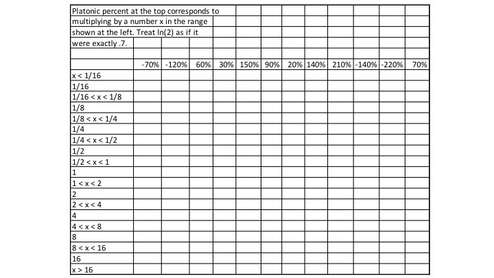
A Platonic change of y% always corresponds to multiplying by exp(.01 y). Approximating ln(2) as if it were exactly .7, this means that a 70% Platonic change corresponds to multiplying by 2. A -70% Platonic change corresponds to multiplying by .5. A 140% Platonic change corresponds to multiplying by 4. In this exercise, you are asked to mark which range the multiplication factor is in for the Platonic percentage changes shown at the top. Please act as if ln(2) were exactly equal to .7 so that a 70% Platonic change is exactly a doubling. 

Notice that a 70% Platonic change is multiplying by 2, which in turn is a 100% Earthly percentage change. A -70% Platonic change is multiplying by .5, which is a -50% Earthly percentage change. One illustration of how Platonic changes can be more convenient that Earthly percentage changes is that a 70% Platonic change followed by a -70% Platonic change gets you back to where you started. But a 100% Earthly percentage change followed by a -100% Earthly percentage change gets you to zero. And a 50% Earthly percentage change followed by a -50% Earthly percentage change gets you a -25% overall Earthly percentage change. 

If you want the exercise as a pdf with the questions on one side and the answers on the other, here it is. Or here it is on this blog post: 

Answers are below.


Returns to Scale Exercise

Let %ΔX be an overall measure of the change in inputs. If each input changes by the same percentage, this is always equal to that percentage change in each input. 

If different inputs change by different percentages, this is a weighted average of the percent changes in each different input. As long as the firm is minimizing costs, the weights will be equal to the share of costs coming from paying for each input:

  • s_K = share_K = RK/(RK+WL) is the cost share of capital (the share of the cost of capital rentals in total cost.)
  • s_L = share_L = WL/(RK+WL) is the cost share of labor (the share of the cost of the wages of labor in total cost.) 

My post "The Shape of Production: Charles Cobb's and Paul Douglas's Boon to Economics" talks about this more in the case of constant-returns-to-scale Cobb-Douglas.

Given %ΔX the degree of returns to scale γ is defined by the equation:

%ΔY = γ %ΔX

if there is no change in technology.

γ = the degree of returns to scale

DON'T CONFUSE SMALL GREEK LETTER γ WITH Y OR y!

The other key equation that you need is 

γ = AC/MC

where 

AC = average cost

MC = marginal cost

Your task in this exercise is to deduce the missing value in each row. One out of AC, MC, %ΔX and %ΔY is missing in each row of the questions. It is there in the answers. The degree of returns to scale γ is never explicitly stated in the row. But since each row assumes no change in technology, 

 γ = AC/MC =  %ΔY / %ΔX

Here is the way to show that  γ = AC/MC. Let C stand for total cost. (Sometimes we use C to stand for "consumption" but not here.) Then if Ω (the capital Greek letter Omega) is a price index for all the factors put together,   

MC = Ω ΔX / ΔY

AC = Ω X/Y

(The changes ΔX and ΔY in the definition of marginal cost stipulate that technology is not changing.) Since the Ω cancels,  

MC/AC = (ΔX/ΔY) / (X/Y)  =  (ΔX/X) / (ΔY/Y) ≈  %ΔX / %ΔY = 1/γ

AC/MC = (X/Y)  / (ΔX/ΔY)   =  (ΔY/Y) / (ΔX/X)  ≈   %ΔY / %ΔX =  γ

The only reason there is an approximation sign is that γ might not be constant. For small changes %ΔX and %ΔY, the degree of returns to scale γ will be approximately constant over the relevant range. For big changes it is some kind of complicated average γ over the relevant range that matters.

Why might γ not be constant? Here is an important case. Suppose there is a fixed cost FC and a constant marginal cost MC, then average cost AC will be declining from a very high level (essentially infinite for tiny amounts of output) toward MC. As the amount of output goes to infinity, the average cost AC converges to the constant marginal cost MC. This makes it clear that γ can't be constant in this case. 

You can either print out this one-sheet pdf file with the questions on one side and the answers on the other side, or you can look at the questions and later on the answers below in this post. Remember that these calculations all assume no change in technology


Student Guest Posts on supplysideliberal.com

Winter Semester, 2014

Winter Semester, 2015

Fall Semester, 2015

Winter Semester, 2016

University of Colorado Boulder, Spring Semester 2018