Logarithms. On Thursday, I let students in my Principles of Macroeconomics class in on the secret that logarithms are the central mathematical tool of macroeconomics. If my memory isn’t playing tricks on me, I can say that in both papers that examine real world data and at least half of macroeconomic theory papers, a logarithm makes an appearance, often in a starring role.  Why are natural logarithms so important?

1. Lesser reason: logarithms can often model how a household or firm makes choices in a particularly simple, convenient way.

2. Greater reason: multiplication and powers appear all the time in macroeconomics. For a price in initial difficulty, logarithms make multiplication and powers and exponential growth look easy.

Among other aspects of making multiplication and powers and exponential growth look easy, logarithms provide a very clean, elegant way of thinking about percent changes.

I am determined to have very few equations in this post, so you will have to depend on your math training for the basic rules of logarithms: how they turn multiplication into addition and powers into multiplication. What I want to accomplish in this post is to give you a better intuitive feel for logarithms–an intuitive feel that math textbooks often don’t provide. I also hope to make a strong connection in your mind between natural logarithms and percent changes.  

One of the most basic uses of logarithms in economics is the logarithmic scale. On a logarithmic scale, the distance between each power of 10 is the same. So the distance from 1 to 10 on the graph is the same as the distance from 10 to 100, which is the same as the distance from 100 to 1000. Here is a link to an example of a graph with a logarithmic scale on the vertical axis I have used before from Catherine Mulbrandon in Visualizing Economics:

• “(Log Scale) Long-term real growth in US GDP 1871-2009."

Contrast that growth line for US GDP to the curve Catherine gets when not using a logarithmic scale on the vertical axis. Here is the link: 

• "Long-term real growth in US GDP 1871-2009."

The idea of the logarithmic scale–which can be boiled down to the idea of always representing multiplication by a given number as the same distance–shows up in two concrete objects, one familiar and one no-longer familiar: pianos and slide rules.

A Piano Keyboard as a Logarithmic Scale. You may not have thought of a piano keyboard as a logarithmic scale, but it is. Including all of the black keys on an equal footing with the white keys, going up one key on the piano is called going up a "semitone.” Going up an octave (say from Low C to Middle C) is going up 12 semitones. And each octave doubles the frequency of the vibrations in a piano string. As explained in the wikipedia article “Piano key frequencies,” at Middle C, the piano string vibrates 261.626 times per second. Each semitone higher on the piano keyboard makes the vibration of the string 1.0594631… times faster. And multiplying by 1.0594631… twelve times is the same as multiplying by 2. The reason our Western musical scale has been designed to have 12 semitones in an octave is interesting. To begin with, two notes whose frequencies have a ratio that is an easy fraction such as 3/2, 5/4 or 6/5 make a pleasing interval. (The Pythagoreans made mathematics part of their religion thousands of years ago partly because of this fact.) Then, it turns out that various powers of 1.0594631… come pretty close to many easy fractions. Here is a table showing the frequencies of various notes relative to the frequency of Middle C, showing some of the easy fractions that come close to various powers of 1.0594631…. A distance of three semitones yields a ratio close to 6/5; a distance of four semitones yields a ratio close to 5/4; a distance of five semitones yields a ratio close to 4/3; and a distance of seven semitones yields a ratio close to 3/2. None of this is exact, but it is all close enough to sound good when the piano is tuned according to this scheme:

Let me bring the discussion back to economics by pointing out that, although interest rates are lower right now, it is not uncommon for the returns on financial investments to multiply savings by something averaging close to 1.059 every year. At typical rates of return for investments bearing some risk, one can think of each year of returns as raising the pitch of one’s funds on average by about one semitone. Starting from Middle C, one can hope to get quite a ways up the piano keyboard by retirement. And savings early in life get raised in pitch a lot more than savings late in life.

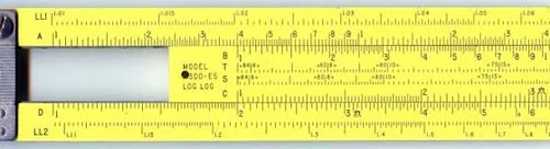
Slide Rules. Slide rules, like the one in the picture right above, are designed first and foremost to use two logarithmic scales that slide along each other to do multiplication. The distances are logarithmic and adding logarithms multiplies the underlying numbers. For example, to multiply 2 times 3,  put the 1 of the sliding piece right at the 3 of the stationary piece. Then look at the 2 on the sliding piece and see what number is next to it on the stationary piece. You could buy a physical slide rule on ebay, but you might instead want to play with a virtual slide rule for free. Playing with this virtual slide rule is one of the best ways to get some intuition for logarithms. (Remember that the distances on a slide rule are all logarithms.) If you like this slide rule and want to go further, here are some much better instructions for using a slide rule than I just gave: Illustrated Self-Guided Course on How to Use the Slide Rule.

Percent Changes (%ΔX). Let me preface what I have to say about percent changes by saying that–other than being a clue that a percent change or a ratio expressed as a percentage lurks somewhere close–I view the % sign as being equivalent to 1/100. So, for example, 23% is just another name for .23, and 100% is just another name for 1. Indeed, economists are just as likely to say “with probability 1” as they are to say “with a 100% probability.”   

It turns out that natural logarithms (“ln” or “log”) are the perfect way to think about percent changes. Suppose a variable X has a “before” and an “after” value.

• I want to take the point of view that the change in the natural logarithm is the pure, Platonic percent change between before and after. It is calculated as the natural logarithm of Xafter minus the natural logarithm of Xbefore.

• I will call the ordinary notion of percent change the earthly percent change. It is calculated as the change divided by the starting value, (Xafter - Xbefore)/Xbefore.

• In between these two concepts is the midpoint percent change. It is calculated as the change divided by the average of the starting and ending values:

(Xafter-Xbefore) / { (Xafter + Xbefore)/2 }

Below is a table showing the relationship between Platonic percent changes, midpoint percent changes and earthly percent changes. In financial terms, one can think of earthly percentage changes as “continuously compounded” versions of Platonic percent changes. Here is the Excel file I used to construct this table that will give you the formulas I used if you want to see them.  

There are at least two things to point out in this table:

1. When the percent changes are small, all three concepts are fairly close, but the midpoint percent change is much closer to the Platonic (logarithmic) percent change.

2. A 70% Platonic percent change is very close to being a doubling–which would be a 100% earthly percent change. This is where the “rule of 70” comes from. (Greg Mankiw talks about the rule of 70 on page 180 of Brief Principles of Macroeconomics.) The rule of 70 is a reflection of the natural logarithm of 2 being equal to approximately .7 = 70%. Similarly, a 140% Platonic percent change is basically two doublings–that is, it is close to multiplying X by a factor of 4; and a 210% Platonic percent change is basically three doublings–that is, it is close to multiplying X by a factor of 8.

Let’s look at negative percent changes as well. Here is the table for how the different concepts of negative percent changes compare:

A key point to make is that with both Platonic (logarithmic) percent changes and midpoint percent changes, equal sized changes of opposite direction cancel each other out. For example, a +50% Platonic percent change, followed by a -50% Platonic percent change, would leave things back where they started. This is true for a +50% midpoint percent change, followed by a -50% midpoint percent change. But, starting from X, a 50% earthly percent change leads to 1.5 X. Following that by a -50% earthly percent change leads to a result of .75 X, which is not at all where things started. This is a very ugly feature of earthly percent changes. That ugliness is one good reason to rise up to the Platonic level, or at least the midpoint level.

Continuous-Time Growth Rates. There are many wonderful things about Platonic percent changes that I can’t go into without breaking my resolve to keep the equation count down. But one of the most wonderful is that to find a growth rate one only has to divide by the time that has elapsed between Xbefore and Xafter. That is, as long as one is using the Platonic percent change %ΔX=log(Xafter)-log(Xbefore),

%ΔX / [time elapsed] = growth rate.

The growth rate here is technically called a “continuous-time growth rate.” The continuous-time growth rate is not only very useful, it is a thing of great beauty.

Update on How the Different Concepts of Percent Change Relate to Each Other.  One of my students asked about how the different percent change concepts relate to each other. For that, I need some equations. And I need “exp” which is the opposite of the natural logarithm “log.” Taking the function exp(X) is the same as taking e, (a number that is famous among mathematicians and equal to 2.718…) to the power X. For the equations below, it is crucial to treat % as another name for 1/100, so that, for example, 5% is the same thing as .05.  

Earthly percent changes are the most familiar. Almost anyone other than an economist who talks about percent changes is talking about earthly percent changes. Most of you learned about earthly percent changes in elementary school. So let me first write down how to get from the earthly percent change to the Platonic and midpoint percent changes. (I won’t try to prove these equations here, just state them.) 

Platonic = log(1 + earthly)

midpoint = 2 earthly/(2 + earthly)

 If you are trying to figure out the effects of continuously compounded interest, or the effects of some other continuous-time growth rate, you will want to be able go from Platonic percent changes–which come straight from multiplying the growth rate by the amount of elapsed time–to earthly percent changes. For good measure, I will include the formula for midpoint percent changes as well:

earthly = exp(Platonic) - 1 

midpoint = 2 {exp(Platonic) - 1}/{exp(Platonic) + 1}

I found the function giving the midpoint percent change as a function of the Platonic percent change quite intriguing. For one thing, when I changed signs and put “-Platonic” in the place where you see “Platonic” on the right-hand side of the equation the result equal to -midpoint. When switching the sign of the argument (the inside thing: Platonic) just switches the sign of the overall expression, mathematicians call it an “odd” function (“odd” as in “odd and even” not “odd” as in “strange”). The meaning of this function being odd is that Platonic and midpoint percent changes map into each other the same way for negative changes as for positive changes.  (That isn’t true at all for the earthly percent changes.) The other intriguing thing about the function giving the midpoint percent change as a function of the Platonic percent change is how close it is to giving back the same number. To a fourth-order (the squared term and the fourth power term are zero), the approximation for the function is this:

midpoint=Platonic - (Platonic cubed/12) + (5th power and higher terms) 

Finally, let me give the equations to go from the midpoint percent change to the Platonic and the     

earthly = 2 midpoint/(2-midpoint)

Platonic = log(2+midpoint) - log(2-midpoint)

             = log(1+{midpoint/2} ) - log(1-{midpoint/2})

The expression for Platonic percent changes in terms of midpoint percent changes has such a beautiful symmetry that its “oddness” is clear. Since I know the way to approximate natural logarithms to as high an order as I want (and I am not special in this), I can give the approximation for Platonic percent changes in terms of powers of midpoint percent changes as follows:

Platonic = midpoint + (midpoint cubed)/12

                   + (midpoint to the fifth power)/80

                   + (midpoint to the seventh power)/448

                   + (9th and higher order terms).

The bottom line is that for even medium-sized percent changes (say 30%), the Platonic percent change is quite close to the midpoint percent change–something the tables above show. By the time the Platonic percent changes and midpoint percent changes start to diverge from each other in any worrisome way, the rule of 70 that makes a 70% Platonic percent change close to equivalent to a doubling starts to kick in to help out.