In my post "There Is No Such Thing as Decreasing Returns to Scale" and my Storify stories "Is There Any Excuse for U-Shaped Average Cost Curves?" and "Up for Debate: There Is No Such Thing as Decreasing Returns to Scale," I criticize U-shaped average cost curves as a staple of intermediate microeconomics classes. But what should be taught in place of U-shaped average cost curves? This post is my answer to that question: returns to scale and imperfect competition in market equilibrium. 

In order to talk about the degree of returns to scale and the degree of imperfect competition, we need a measure of each. The following notation is helpful:

The Degree of Returns to Scale

The degree of returns to scale can be measured by the percent change in output for a 1% change in inputs. I use the Greek letter gamma for the degree of returns to scale:

when there is only a single input in the amount x. (Note that throughout this post I use the percent change concepts and notation from "The Logarithmic Harmony of Percent Changes and Growth Rates" and write as equalities approximations that are very close when changes are small.) 

According to the awkward, but traditional terminology, a degree of returns to scale equal to one is "constant returns to scale." A degree of returns to scale greater than one is "increasing returns to scale." As for a degree of returns to scale less than one, make sure to read "There Is No Such Thing as Decreasing Returns to Scale."

If more than one input is used to produce the firm's output, a convenient way to gauge the increase in inputs is to look at the change in total cost holding factor prices fixed. This gives an aggregate of all the different factors weighted by the initial factor prices. Notice that for the standard production technology notion of returns to scale it doesn't matter if factor prices are actually unchanging as the firm changes its level of output; holding factor prices fixed is simply a way to get an index for total factor quantities akin to the way real GDP is measured. Using the percent change in total cost with factor prices held fixed to gauge the percent change in inputs, the degree of returns to scale with multiple factors is:

Remember that this equation is about what happens when a firm changes the quantity of its output, always producing that output in a minimum cost way given those fixed factor prices. If factor prices or technology are changing, then this equation does not hold. 

I argue that the degree of returns to scale will typically be declining in the quantity of output. I base this in part on the idea that a fixed cost coupled with a constant marginal cost is the base case we should start from as economists. Here is why the degree of returns to scale declines with the level of output when a firm has a fixed cost coupled with a constant marginal cost: 

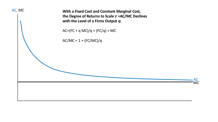
According to the derivation above, the degree of returns to scale gamma is equal to AC/MC. Thus, when a firm has a fixed cost coupled with a constant marginal cost for the product whose cost is depicted, the degree of returns to scale declines with the level of the output for that product. What is more, if marginal cost MC is constant, the degree of returns to scale gamma = AC/MC has the same shape as the average cost curve AC, though the vertical scale for the degree of returns to scale would have 1 in place of MC. 

The Degree of Imperfect Competition

The degree of imperfect competition can be measured by how far above its marginal revenue a firm will want to set its price: the desired markup ratio p/MR. I use the Greek letter mu for the desired markup ratio. Since a firm tries to set its price so that marginal revenue equals marginal cost, this is also how far above its marginal cost a firm will want to set is price. This actual markup ratio p/MC can be different from the desired markup ratio p/MR over periods of time when the firm doesn't have full price flexibility, but in long-run equilibrium, the actual markup ratio P/MC should be equal to the desired markup ratio p/MR.  

The desired markup ratio that measures the degree of imperfect competition is closely related to the price elasticity of demand a firm faces, but goes up when the price elasticity of demand the firm faces goes down. I use the Greek letter epsilon for the price elasticity of demand faced by a firm. The key identity can be derived as follows:

Here is a table giving the desired markup ratio for various values of the price elasticity of demand faced by a firm:

Price Elasticity of Demand Faced by a Firm epsilon    Desired Markup Ratio mu

                                         1                                                            infinity

                                         1.5                                                         3

                                         2                                             2

                                         2.5                                          1.67

                                         3                                             1.5

                                         4                                             1.33

                                         5                                             1.25

                                         6                                             1.2

                                         7                                             1.17

                                         8                                             1.14

                                        10                                            1.11

                                        11                                              1.1 

                                        21                                              1.05 

                                       101                                             1.01

                                    infinity                                          1                                        

There are several noteworthy aspects about this table. First, if a firm has a marginal cost of zero, in long-run equilibrium it will seek out a price at which the price elasticity of demand it faces is equal to 1. The infinite markup ratio corresponds to a positive price divided by a zero marginal cost. I plan to talk about the market equilibrium for this case in a future post. 

If a firm has any positive marginal cost, then in long-run equilibrium, regardless of what other firms do, it will keep raising its price until it reaches a price at which the price elasticity of demand it faces is greater than 1, unless it can get away with providing an infinitesimal quantity at an infinite price. (Being able to get away with providing an infinitesimal quantity at an infinite price is unlikely.) Therefore with a positive marginal cost, the desired markup ratio will be finite and greater than one.

A higher desired markup ratio corresponds a lower price elasticity of demand. And a higher desired markup ratio corresponds to more imperfect competition. The desired markup ratio is a very convenient way to measure the degree of imperfect competition.

Market Equilibrium

The graph at the top of this post illustrates market equilibrium. I return to that graph below. For the logic behind market equilibrium, let me quote from my paper "Next Generation Monetary Policy": 

Given free entry and exit of monopolistically competitive firms, in steady state average cost (AC) should equal price (P): if P > AC, there should be entry, while if P < AC there should be exit, leading to P=AC in steady state. Price adjustment makes marginal cost equal to marginal revenue in steady state. Thus, with free entry, in steady state,

where by a useful identity γ is equal to the degree of returns to scale and μ is a bit of notation for the desired markup ratio P/MR. The desired markup ratio is equal in turn to the price elasticity of demand epsilon divided by epsilon minus one: 

Remarkably, in long-run equilibrium, after both price adjustment and entry and exit, the degree of returns to scale must be equal to the degree of imperfect competition as measured by the desired markup. 

I am going to make four key simplifications to make it easier to understand market equilibrium. First, I will assume that the market equilibrium is symmetric so that each firm sells the same amount q. Second, I will assume, at least for the benchmark case that the elasticity of demand for the entire industry's output is zero. That is, customers are perfectly happy to shift from buying one firm's output to buying another firm's output at the elasticity epsilon if they can get a better deal, but they insist on a certain amount of the category of good provided by the industry. Using the letter Q for the total sales in the industry, that means

Q=nq

n=Q/q

q=Q/n 

Third, I will assume that the price elasticity of demand a firm faces—and therefore its desired markup ratio—depends only on the number of firms in the industry. Fourth, I will assume that all fixed costs are flow fixed costs rather than being sunk. It is interesting to relax each of these assumptions, but it would be hard to understand those cases without first learning the simplified case I am presenting here. (The most difficult to relax is the symmetry assumption. Relaxing that assumption is least likely to meet the cost-benefit test in the tradeoff between tractability and realism.)

Let me reprise the graph at the top of this post to explain how it illustrates market equilibrium:

This graph is really two interlocking graphs. On the right, the degree of returns to scale and the degree of imperfect competition as measured by the desired markup ratio are shown in relation to the output of a typical firm. On the left, the degree of returns to scale and the degree of imperfect competition as measured by the desired markup ratio are shown in relation to the number n of firms in the industry. 

The degree of returns to scale declines with output as explained above. For given total sales in the industry Q, that means that the degree of returns to scale increases with the number of firms in the industry. 

The degree of imperfect competition as measured by the desired markup ratio decreases with the number n of firms in the industry. For given total sales in the industry Q, that means that the degree of imperfect competition as measured by the desired markup ratio increases with a typical firm's output q.

The assumption that—other things equal—the degree of imperfect competition declines with the number of firms is intuitive—and I believe correct in the real world. But I should note that there is a very popular model—the Dixit-Stiglitz model—that is popular in important measure because it makes the degree of imperfect competition as measured by the desired markup ratio constant, regardless of how many or few firms there are. The Salop model gives a degree of imperfect competition as measured by the desired markup ratio that declines with the number of firms. But the Salop model is less convenient technically than the Dixit-Stiglitz model. Innovation could be valuable here. A model that had an attractive story, was technically convenient and had a desired markup ratio declining in the number of firms should be able to attract a subsantial number of users. In any case, I stand by the claim that to model the real world, one should have the desired markup ratio declining in the number of firms in the industry.    

The intersection on the right shows the long-run equilibrium output of a typical firm in this industry. The intersection on the left shows the long-run equilibrium number of firms in the industry.

When mu > gamma.  Though this could be questioned, think of entry and exit happening at a slower pace than price adjustment. (I discuss the relationship between some other adjustment speeds in "The Neomonetarist Perspective.") Once prices have adjusted, MC = MR. So if the degree of imperfect competition mu = p/MR is greater than the degree of returns to scale gamma = AC/MC it means that p > AC and there will be entry. As n rises, AC and p will come closer together until they are equal at the intersection on the left side of the graph.

When mu < gamma.  On the other hand, If the degree of imperfect competition mu = p/MR is less than the degree of returns to scale gamma = AC/MC, it means that p < AC and there will be exit. As n falls, AC and p will come closer together until they are equal at the intersection on the left side of the graph.

To summarize:

• If mu > gamma, firms enter.

• If gamma > mu, firms exit.

In either case, as n adjusts, the quantity of a typical firm's output also changes. 

Comparative Statics

Let's consider four thought experiments. First, consider an increase in total sales Q by the industry. This shifts out both curves that are written in terms of Q:

The prediction is that both the number of firms and the output of a typical firm will increase, while both the degree of returns to scale and the degree of imperfect competition will fall. Because the curve showing the desired markup as a function of the number of firms does not shift, the reduction in the the desired markup only occurs as new firms actually enter. The degree of returns to scale overshoots: it drops most right after the increase in total industry sales Q, then gradually rises again as new firms enter and the quantity produced by each firm declines. 

Second, consider reduction in the (flow) fixed cost. This cases the returns to scale (gamma) curves on both sides to shift downward:

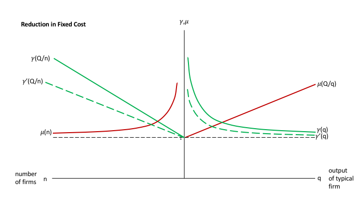
The prediction is that the number of firms will increase, while the size of a typical firm decreases, and that both the degree of returns to scale and the degree of imperfect competition will fall. Because the desired markup curves does not shift, the desired markup only falls as new firms actually enter, which is likely to be gradual. As in the first experiment, the degree of returns to scale overshoots in the sense of dropping most at first. 

With the marginal cost unchanged, the fall in the desired markup ratio leads to a reduction in price. That would expand the size of the industry if the elasticity of demand for the industry product category as a whole were nonzero. That in turn would require the results of the first experiment in order to analyze.

Third, consider a reduction in marginal cost. This causes the returns to scale curves on both sides to shift up, since returns to scale equals AC/MC, and because it includes average fixed cost, AC does not fall as much as MC. However, the effect of MC on AC means that the gamma = AC/MC curves do not rise vertically by as large a percentage as MC falls. 

The prediction is that the output of a typical firm will rise, while the number of firms will decline. The degree of returns to scale and degree of imperfect competition rise in the long run. But note that this is because of improved performance of the industry in reducing costs. The equilibrium desired markup ratio rises less than the degree of returns to scale curve, which in turn rises by a smaller percentage than MC falls. The price will be lowest before firms have had a chance to exit—indeed it will initially fall by the full percentage of the decline in MC—but will remain lower in the new long-run equilibrium than in the old long-run equilibrium.

Again, if the elasticity of demand for industry output as a whole is nonzero, the decline in price would lead Q to increase (more at first, somewhat less later on), so the results of the first experiment would be necessary to fully analyze what would happen.  

Fourth, consider an increase in the price elasticity of demand for any given number of firms. This might be described as the market becoming "more price-competitive." Both desired markup curves fall: 

The prediction is that in the long run the number of firms falls, while the output of the typical firm rises. This might be called a "shakeout" of the industry. Because the industry has become more price-competitive, the number of firms falls. Someone coming from the ancient "Structure-Conduct-Performance" paradigm for Industrial Organization might be confused because the concentration of the industry goes up, yet the performance of the industry improves: the degree of imperfect competition as measured by the desired markup falls, as does the degree of returns to scale in long-run equilibrium.

With MC unchanged, the desired markup and therefore the price falls most right at first, before firms have had a chance to exit. Then the price comes up somewhat, but remains lower than in the initial long-run equilibrium. If the price elasticity of demand for the entire industry's output is nonzero, then Q will increase, especially at first, which will complicate the analysis in ways that the first experiment can help navigate. 

Conclusion

In my view, the foregoing analysis is

• more on-target than U-shaped average cost curves in relation to the real world

• more interesting than U-shaped average cost curves

• no harder than U-shaped average cost curves, if one sticks to the simplifications I made. What I have laid out above is difficult, but U-shaped average cost curves are also difficult.

Therefore, it seems better to me to teach returns to scale and imperfect competition in market equilibrium than it is to teach U-shaped average cost curves. In any case, there are always tradeoffs. When it is impossible to teach both, what I have laid out in this post is the opportunity cost for teaching U-shaped average cost curves. I hope you will agree it represents a high opportunity cost, indeed.