
Where is Social Science Genetics Headed?


Social science genetics is on the rise. The article shown above is a recent triumph. By knowing someone’s genes alone, it is possible to predict 11–13% of the number of years of schooling they have. Such a prediction comes from adding up tiny effects of many, many genes.
Since a substantial fraction of my readers are economists, let me mention that some of the important movers and shakers in social science genetics are economists. For example, behind some of the recent successes is a key insight, which David Laibson among others had to defend vigorously to government research funders: large sample sizes were so important in accurately measuring the effects of genes that it was worth sacrificing quality of an outcome variable if that would allow a much larger sample size. Hence, when they were doing the kind of research illustrated by the article shown above, it was a better strategy to put the lion’s share of effort into genetic prediction of number of years of education than genetic prediction of intelligence, simply because number of years of education was a variable collected along with genetic data for many more people than intelligence was.
One useful bit of terminology for genetics is that other non-genetic information about an individual, such as years of education or blood pressure are called “phenotypes.” Another is that linear combinations of data across many genes intended to be best linear predictors of a particular phenotype are called “polygenic scores.” Polygenic scores have known signal-to-noise ratios, making it possible to do measurement-error corrections for their effects. (See “Adding a Variable Measured with Error to a Regression Only Partially Controls for that Variable” and “Statistically Controlling for Confounding Constructs is Harder than You Think—Jacob Westfall and Tal Yarkoni.”)
Both private companies and government-supported initiatives around the world are rapidly increasing the amount of human genotype data linked to other data (with a growing appreciation of the need for large samples of people over the full range of ethnic origins). For common variations (SNPs) that have well-known short-range correlations, genotyping using a chip now costs about $25 per person when done in bulk, while “sequencing” to measure all variations, including rare ones, costs about $100 per person, with the costs rapidly coming down. Sample sizes are already above a million individuals, with concrete plans for several million more that will be data sets that are quite accessible to researchers.
In this post, I want to forecast where social science genetics is headed in the next few years. I don’t think I am sticking my neck out very much with these forecasts about cool things people will be doing. Those in the field might say “Duh. Of course!” Here are some types of research I think will be big:
Genetic Causality from Own Genes and Sibling Effects. Besides increasing the amount of data on non-European ethnic groups, a key direction data collection will move in the future is to collect genetic data on mother-father-self trios and mother-father-self-sibling quartets. (For example, the PSID is now in the process of collecting genetic data.) Conditional on the mother’s and father’s genes, both one’s own genes and the genes of a full sibling are as random as a coin toss. As a result, given such data, one can get clean causal estimates of the effects of one’s own genes on one’s outcomes and the effects of one’s sibling’s genes on one’s outcomes.
Genetic Nurturance. By looking at the genes of the mother and father that were not transmitted to self, one can also get important evidence on the effects of parental genes on the environment parents are providing. (Here, the evidence is not quite as clean. Everything the non-transmitted parental genes are correlated with could be having a nurture effect on self.) Effects of nontransmitted parental genes are interesting because most things that parents can do other than passing on their genes are things a policy intervention could imitate. That is, the effects of non-transmitted parental genes reflect nurture.
Recognizing Faulty Identification Claims that Involve Genetic Data. One reason expertise in social science genetics is valuable is that questionable identification claims will be made and are being made involving genetic data. While the emerging data will allow very clean identification of causal effects of genes on a wide range of outcomes, the pathway by which genes have their effects can be quite unclear. People will make claims that genes are good instruments. This is seldom true, because the exclusion restriction that genes only act through a specified set of right-hand side variables is seldom satisfied. Also, it is important to realize that large parts of the causal chain are likely to go through the social realm outside an individual’s body.
Treatment Effects that Vary by Polygenic Score. One interesting finding from research so far is that treatment effects often differ quite a bit when the sample is split by a relevant polygenic score. For example, effects of parental income on years of schooling are more important for women who have low polygenic scores for educational attainment. That is, women who have genes predicting a lot of education will get a lot of education even if parental income is low, but women whose genes predict less education will get a lot of education only if parental income is high. The patterns are different for men.
Note that treatment effects varying by polygenic score has obvious policy implications. For example, suppose we could identify kids in very bad environments who had genes suggesting they would really succeed if only they were given true equality of opportunity. This would sharpen the social justice criticism of the lack of opportunity they currently have. Notice that many of the policy implications based on treatment effects that vary by polygenic score would be highly controversial, so knowledge of the ins and outs of ethical debates about the use of genetic data in this way becomes quite important.
Enhanced Power to Test Prevention Strategies. One unusual aspect of genes is that the genetic data, with all the predictive power that provides, are available from the moment of birth and even before. This means that prevention strategies (say for teen pregnancy, teen suicide, teen drug addiction or being a high school dropout) can be tested on populations whose genes indicated elevated risk, which could dramatically increase power for field experiments.
The Option Value of Genetic Data. Suppose one is doing a lab experiment with a few hundred participants. With a few thousand dollars, one could collect genetic data. With that data, one could immediately begin to control for genetic differences that contribute to standard errors and look at differences in treatment effects on experimental subjects who have different polygenic scores. But with the same data, one would also be able to do a new analysis four years later using more accurate polygenic scores or using polygenic scores that did not exist earlier. In this sense, genetic data grows in value over time.
The example above was with genetic data in a computer file that can be combined with coefficient vectors to get improved or new linear combinations. If one is willing to hold back some of the genetic material for later genetic analysis with future technologies (as the HRS did), totally new measurements are possible. For example, many researchers have become interested in epigenetics—the methylation marks on genes that help control expression of genes.
Assortative Mating. Ways of using genetic data that are not about polygenic scores in a regression will emerge. My own genetic research—working closely with Patrick Turley and Rosie Li—has been about using genetic data on unrelated individuals to look at the history of assortative mating. Genetic assortative mating for a polygenic score is defined as a positive covariance between the polygenic scores of co-parents. But one need not have direct covariance evidence. A difference equation indicates that a positive covariance between the polygenic scores of co-parents shows up in a higher variance of the polygenic scores of the children. Hence, data on unrelated individuals shows the assortative mating covariance among the parents’ generation in the birth-year of those on whom one has data. One can go further. When a large fraction of a population is genotyped, the genetic data can, itself, identify cousins. This makes it possible to partition people’s genetic data in a way that allows one to measure assortative mating in even earlier generations.
Conclusion: Why More and Better Data Will Make Amazing Things Possible in Social Science Genetics. One interesting thing about genetic data is that, there is a critical sample size at which it is possible to get good accuracy on the genes for any particular outcome variable. Why is that? after multiple-hypothesis-testing correction for the fact that there are many, many genes being tested, “genome-wide significance” requires a z-score of 5.45. (Note that, with large sample sizes, the z-score is essentially equal to the t-statistic.) But a characteristic of the normal distribution is that at such high z-score, even a small change in z-score can make a huge difference in p-value. A t-score of 5.03 has a p-value ten times as big, and a score of 5.85 has a p-value ten times smaller. That means that in this region, for a given coefficient estimate an 18% increase in sample size is guaranteed to change a p-value by an order of magnitude. Thinking about things the other way around, if there are genes with different sizes of effects distributed normally, if to start with, one can only reliably detect things far out on the normal distribution of effect sizes, then a modest percentage increase in sample size will make a bigger slice of the normal distribution of effect sizes reliably detectable, which will mean identifying many times as many genes as genome-wide significant.
The critical sample size depends on what phenotype one is looking at. Most importantly, power is lower for diseases or other conditions that are relatively rare. The critical sample size at which we will get a good polygenic score for anorexia is much larger than the sample size at which one can get a good polygenic score for educational attainment. But as sample sizes continue to increase, at some point, relatively suddenly, we will be there with a good polygenic score for anorexia. Just imagine if parents knew in advance that one of their children was at particularly high risk for anorexia. They’d be likely to do things differently and might be able to avert that problem.
I am sure there are many cool things in the future of social science genetics that I can’t imagine. It is an exciting field. I am delighted to be along for the ride!
Here are some other posts on genetic research:
Randolph Nesse on Efforts to Prevent Drug Addiction
Criminalization and interdiction have filled prisons and corrupted governments in country after country. However, increasingly potent drugs that can be synthesized in any basement make controlling access increasingly impossible. Legalization seems like a good idea but causes more addiction. Our strongest defense is likely to be education, but scare stories make kids want to try drugs. Every child should learn that drugs take over the brain and turn some people into miserable zombies and that we have no way to tell who will get addicted the fastest. They should also learn that the high fades as addiction takes over.
New treatments are desperately needed.
—Randolph Nesse, Good Reasons for Bad Feelings, in Chapter 13, “Good Feelings for Bad Reasons.”
What is the Evidence on Dietary Fat?

Based on an article in “Obesity Reviews” by Santos, Esteves, Pereira, Yancy and Nunes entitled “Systematic review and meta-analysis of clinical trials of the effects of low carbohydrate diets on cardiovascular risk factors,” lowcarb diets look like (on average) they reduce
weight
abdominal circumference
systolic and diastolic blood pressure
blood triglycerides
blood glucose
glycated hemoglobin,
insulin levels in the blood,
C-reactive protein
while raising HDL cholesterol (“good cholesterol”). But lowcarb diets don’t seem to reduce LDL cholesterol (“bad cholesterol”). This matches my own experience. In my last checkup my doctor said all of my blood work looked really good, but that one of my cholesterol numbers was mildly high.
Nutritionists often talk about the three “macronutrients”: carbohydrates, protein and fat. For nutritional health, many of the most important differences are within each category. Sugar and easily-digestible starches like those in potatoes, rice and bread are very different in their health effects than resistant starches and the the carbs in leafy vegetables. Animal protein seems to be a cancer promoter in a way that plant proteins are not. (And non-A2 cow’s milk contains a protein that is problematic in other ways.) Transfats seem to be quite bad, but as I will discuss today, there isn’t clear evidence that other dietary fats are unhealthy.
Between the three macronutrients, I think dietary fat doesn’t deserve its especially bad reputation—and protein doesn’t deserve its especially good reputation. Sugar deserves an even worse reputation than it has, but there are other carbs that are OK. Cutting back on bad carbs usually goes along with increasing either good carbs, protein or dietary fat. Many products advertise how much protein they have; but that is not necessarily a good thing.
Besides transfats, which probably deserve their bad reputation, saturated fats have the worst reputation among dietary fats. So let me focus on the evidence about saturated fat. One simple point to make is that saturated fats in many meat and dairy products tend to come along with animal protein. As a result, saturated fat has long been in danger of being blamed for crimes by animal protein. Butter doesn’t have that much protein in it, but tends to be eaten on top of the worst types of carbs, and so is in danger of being blamed for crimes by very bad carbs.
Part of the conviction that saturated fat is unhealthy comes from the effect of eating saturated fat on blood cholesterol levels. So any discussion of whether saturated fat is bad has to wrestle with the question of how much we can infer from effects on blood cholesterol. One of the biggest scientific issues there is that the number of different subtypes of cholesterol-transport objects in the bloodstream is considerably larger than the number of quantities that are typically measured. It isn’t just HDL cholesterol, tryglicerides and LDL cholestoral numbers that matter. The paper shown at the top of this post, “Systematic review and meta-analysis of clinical trials of the effects of low carbohydrate diets on cardiovascular risk factors,” explains:
Researchers now widely recognise the existence of a range of LDL particles with different physicochemical characteristics, including size and density, and that these particles and their pathological properties are not accurately measured by the standard LDL cholesterol assay. Hence assessment of other atherogenic lipoprotein particles (either LDL alone, or non-HDL cholesterol including LDL, intermediate density lipoproteins, and very low density lipoproteins, and the ratio of serum apolipoprotein B to apolipoprotein A1) have been advocated as alternatives to LDL cholesterol in the assessment and management of cardiovascular disease risk. Moreover, blood levels of smaller, cholesterol depleted LDL particles appear more strongly associated with cardiovascular disease risk than larger cholesterol enriched LDL particles, while increases in saturated fat intake (with reduced consumption of carbohydrates) can raise plasma levels of larger LDL particles to a greater extent than smaller LDL particles. In that case, the effect of saturated fat consumption on serum LDL cholesterol may not accurately reflect its effect on cardiovascular disease risk.
In brief, the abundance of cholesterol-transport object subtypes whose abundance isn’t typically measured separately could matter a lot for health. Some drugs that reduce LDL help reduce mortality; others don’t. The ones that reduce mortality could be reducing LDL by reducing some of the worst subtypes of cholesterol-transport objects, while the ones that don’t work could be reducing LDL by reducing some relatively innocent subtypes of cholesterol-transport objects. As Santos, Esteves, Pereira, Yancy and Nunes write in the article shown at the top of this post:
As the diet-heart hypothesis evolved in the 1960s and 1970s, the focus shifted from the effect of dietary fat on total cholesterol to LDL cholesterol. However, changes in LDL cholesterol are not an actual measure of heart disease itself. Any dietary intervention might influence other, possibly unmeasured, causal factors that could affect the expected effect of the change in LDL cholesterol. This possibility is clearly shown by the failure of several categories of drugs to reduce cardiovascular events despite significant reductions in plasma LDL cholesterol levels.
Another way to put the issue is that cross-sectional variation in LDL (“bad”) cholesterol levels for which higher LDL levels look bad for health may involve a very different profile of changes in cholesterol-transport object subtypes than eating more saturated fats from coconut milk, cream or butter would cause (in the absence of the bad carbs such as bread or potatoes that often go along with butter). Likewise, variation in LDL (“bad”) cholesterol levels associated with statin treatment in which statin drugs look good for reducing mortality may may involve a very different profile of changes in cholesterol-transport object subtypes than eating more saturated fats from coconut milk, cream or butter itself would cause.
The article “Systematic review and meta-analysis of clinical trials of the effects of low carbohydrate diets on cardiovascular risk factors” gives an excellent explanation of the difficulty in getting decisive evidence about the effects of eating saturated fat on disease. The relevant passage deserves to be quoted at length:
These controversies arise largely because existing research methods cannot resolve them. In the current scientific model, hypotheses are treated with scepticism until they survive rigorous and repeated tests. In medicine, randomised controlled trials are considered the gold standard in the hierarchy of evidence because randomisation minimises the number of confounding variables. Ideally, each dietary hypothesis would be evaluated by replicated randomised trials, as would be done for the introduction of any new drug. However, this is often not feasible for evaluating the role of diet and other behaviours in the prevention of non-communicable diseases.
One of the hypotheses that requires rigorous testing is that changes in dietary fat consumption will reduce the risk of non-communicable diseases that take years or decades to manifest. Clinical trials that adequately test these hypotheses require thousands to tens of thousands of participants randomised to different dietary interventions and then followed for years or decades until significant differences in clinical endpoints are observed. As the experience of the Women’s Health Initiative suggests, maintaining sufficient adherence to assigned dietary changes over long periods (seven years in the Women’s Health Initiative) may be an insurmountable problem. For this reason, among others, when trials fail to confirm the hypotheses they were testing, it is impossible to determine whether the failure is in the hypothesis itself, or in the ability or willingness of participants to comply with the assigned dietary interventions. This uncertainty is also evident in diet trials that last as little as six months or a year.
In the absence of long term randomised controlled trials, the best available evidence on which to establish public health guidelines on diet often comes from the combination of relatively short term randomised trials with intermediate risk factors (such as blood lipids, blood pressure, or body weight) as outcomes and large observational cohort studies using reported intake or biomarkers of intake to establish associations between diet and disease. Although a controversial practice, many, if not most, public health interventions and dietary guidelines have relied on a synthesis of such evidence. Many factors need to be considered when using combined sources of evidence that individually are inadequate to formulate public health guidelines, including their consistency and the likelihood of confounding, the assessment of which is not shared universally. The level of evidence required for public health guidelines may differ depending on the nature of the guideline itself.
That is the state of the solid evidence. In terms of common notions that many people, including doctors, have in their heads, one should be aware of the hysteresis (lock-in from past events) in attitudes toward fat. Techniques of measuring overall cholesterol concentrations in the blood became possible in the early 20th century. Tentative conclusions reached then based on what would now clearly be recognized as a too-low-dimensional measurement of cholesterol have continued to effect attitudes even now, the better part of a century later. And the decision of the McGovern committee on dietary guidelines to advise against dietary fat rather than advise against sugar—which was a nonobvious duel among competing experts at the time—became dogma for a long time. Thankfully, the idea that dietary fat is worse than sugar is weakening as a dogma, so there is a chance now for scientific evidence to play a decisive role. If only solid evidence were easier to come by!
No one knows the truth of the matter about dietary fat. And many doctors know less then you do now if you have made it to the end of this post. Where have I placed my bets? Eliminating sugar and other bad carbs from my diet would make my diet too bland for comfort if I didn’t allow a lot of fats. I eat a lot of avocados and a lot of olive oil, which most experts think have quite good fats. (See “In Praise of Avocados.”) But I also eat quite a bit of coconut milk, cream and butter (without the bread or potatoes!) I don’t know if that is OK, but I feel quite comfortable doing so.
In addition to all of the evidentiary problems mentioned above, very few clinical trials look at the effects of what kinds of fats people eat when they are fasting regularly (that is, going without food for extended periods of time). It may be just my optimism, but if saturated fats do have some bad effects, I have some hope that fasting gives my body time to repair any damage that may result.
I dream of a day when there will be funds to do types of dietary research that have been underdone. I think research funding has been skewed toward cure of diseases people already have over research that can help prevention. Hopefully, that skewing will someday be rectified.
For annotated links to other posts on diet and health, see:
Miles Kimball on John Locke's Second Treatise

I have finished blogging my way through John Locke’s Second Treatise on Government: Of Civil Government, just as I blogged my way through John Stuart Mill’s On Liberty. (See “John Stuart Mill’s Defense of Freedom” for links to those posts.) These two books lay out the main two philosophical approaches to defending freedom: John Stuart Mill’s Utilitarian approach and John Locke’s Natural Rights approach. To me, both of these approaches are appealing, though I lean more to the Utilitarian approach. One way in which I combine these two approaches is by maintaining that no government action that clearly both reduces freedom and lowers overall social welfare is legitimate, regardless of what procedural rules have been followed in its enactment.
In my blog posts about John Locke’s Second Treatise on Government: Of Civil Government and John Stuart Mill’s On Liberty I am not afraid to disagree with John Locke or John Stuart Mill. But I find myself agreeing with each of them much more than I disagree. My own love of and devotion to freedom is much stronger as a result of blogging through these two books. I am grateful to be a citizen of the United States of America, which was, in important measure, founded on the ideas laid out by John Locke. If the United States of America is true to its founding conception, it will be a land of even greater freedom in the future than it is now.
I have organized my blog posts on John Locke’s Second Treatise on Government: Of Civil Government according to five sections of the book. Each of the following is a bibliographic post with links to the posts on that section.
Links to Posts on Chapters I–III: John Locke's State of Nature and State of War
Links to Posts on Chapters IV–V: On the Achilles Heel of John Locke's Second Treatise: Slavery and Land Ownership
Links to Posts on Chapters VI–VII : John Locke Against Natural Hierarchy
Links to Posts on Chapters VIII–XI: John Locke's Argument for Limited Government
Links to Posts on Chapters XII–XIX: John Locke Against Tyranny
In addition to the links within the posts above traversing the Second Treatise in order, I have one earlier post based on John Locke's Second Treatise:
Statistically Controlling for Confounding Constructs is Harder than You Think—Jacob Westfall and Tal Yarkoni

Last week, I posted “Adding a Variable Measured with Error to a Regression Only Partially Controls for that Variable.” Today, to reinforce that message, I’ll discuss the PlosOne paper “Statistically Controlling for Confounding Constructs is Harder than You Think” (ungated), by Jacob Westfall and Tal Yarkoni. All the quotations in this post come from that article. (Both Paige Harden and Tal Yarkoni himself pointed me to this article.)
A key bit of background is that social scientists are often interested not in just prediction, but in understanding. Jacob and Tal write:
To most social scientists, observed variables are essentially just stand-ins for theoretical constructs of interest. The former are only useful to the extent that they accurately measure the latter. Accordingly, it may seem natural to assume that any statistical inferences one can draw at the observed variable level automatically generalize to the latent construct level as well. The present results demonstrate that, for a very common class of incremental validity arguments, such a strategy runs a high risk of failure.
What is “incremental validity”? Jacob and Tal explain:
When a predictor variable in a multiple regression has a coefficient that differs significantly from zero, researchers typically conclude that the variable makes a “unique” contribution to the outcome.
“Latent variables” are the underlying concepts or “constructs” that social scientists are really interested in. This passage distinguishes latent variables from the “proxies” actually in a data set:
And because measured variables are typically viewed as proxies for latent constructs of substantive interest … it is natural to generalize the operational conclusion to the latent variable level; that is, to conclude that the latent construct measured by a given predictor variable itself has incremental validity in predicting the outcome, over and above other latent constructs that were examined.
However, this is wrong, for the reason stated in the title of my post: “Adding a Variable Measured with Error to a Regression Only Partially Controls for that Variable.” Here, it is crucial to realize that any difference between the variable actually available in a data set and the underlying concept it is meant to proxy for counts as “measurement error.”
How bad is the problem?
The scope of the problem is considerable: literally hundreds of thousands of studies spanning numerous fields of science have historically relied on measurement-level incremental validity arguments to support strong conclusions about the relationships between theoretical constructs. The present findings inform and contribute to this literature—and to the general practice of “controlling for” potential confounds using multiple regression—in a number of ways.
Unless a measurement error model is used, or a concept is measured exactly, the words “controlling for” and “adjusting for” are red flags for problems:
… commonly … incremental validity claims are implicit—as when researchers claim that they have statistically “controlled” or “adjusted” for putative confounds—a practice that is exceedingly common in fields ranging from epidemiology to econometrics to behavioral neuroscience (a Google Scholar search for “after controlling for” and “after adjusting for” produces over 300,000 hits in each case). The sheer ubiquity of such appeals might well give one the impression that such claims are unobjectionable, and if anything, represent a foundational tool for drawing meaningful scientific inferences.
Unfortunately, incremental validity claims can be deeply problematic. As we demonstrate below, even small amounts of error in measured predictor variables can result in extremely poorly calibrated Type 1 error probabilities.
…
… many, and perhaps most, incremental validity claims put forward in the social sciences to date have not been adequately supported by empirical evidence, and run a high risk of spuriousness.
The bigger the sample size, the more confidently researchers will assert things that are wrong:
We demonstrate that the likelihood of spurious inference is surprisingly high under real-world conditions, and often varies in counterintuitive ways across the parameter space. For example, we show that, because measurement error interacts in an insidious way with sample size, the probability of incorrectly rejecting the null and concluding that a particular construct contributes incrementally to an outcome quickly approaches 100% as the size of a study grows.
The fundamental problem is that the imperfection in variables actually in data sets as proxies for the concepts of interest doesn’t make it harder to know what is going on, it biases results. If researchers treat proxies as if they were the real thing, there is trouble:
In all of these cases—and thousands of others—the claims in question may seem unobjectionable at face value. After all, in any given analysis, there is a simple fact of the matter as to whether or not the unique contribution of one or more variables in a regression is statistically significant when controlling for other variables; what room is there for inferential error? Trouble arises, however, when researchers behave as if statistical conclusions obtained at the level of observed measures can be automatically generalized to the level of latent constructs [9,21]—a near-ubiquitous move, given that most scientists are not interested in prediction purely for prediction’s sake, and typically choose their measures precisely so as to stand in for latent constructs of interest.
Jacob and Tal have a useful section in their paper on statistical approaches that can deal with measurement error under assumptions that, while perhaps not always holding, are a whole lot better than the assumption than assuming a concept is measured precisely by the proxy in the data for that concept. They also make the point that, after correctly accounting for measurement error—including any differences between what is in the data and the underlying concept of interest—often there is not enough statistical power in the data to say much of anything. That is life. Researchers should be engaging in collaborations to get large data sets that—properly analyzed with measurement error models—can really tell us what is going on in the world, rather than using data sets they can put together on their own that are too small to reliably tell what is going on. (See “Let's Set Half a Percent as the Standard for Statistical Significance.” Note also that preregistration is one way to make results at a less strict level of statistical significance worth taking seriously.) On that, I like the image at the top of Chris Chambers’s Twitter feed:

Dan Benjamin, my coauthor on many papers, and a strong advocate for rigorous statistical practices that can really help us figure out how the world works, suggested the following two articles as also relevant in this context:

Here are links to other posts that touch on statistical issues:
Adding a Variable Measured with Error to a Regression Only Partially Controls for that Variable
Let's Set Half a Percent as the Standard for Statistical Significance
Less Than 6 or More than 9 Hours of Sleep Signals a Higher Risk of Heart Attacks
Eggs May Be a Type of Food You Should Eat Sparingly, But Don't Blame Cholesterol Yet
Henry George Eloquently Makes the Case that Correlation Is Not Causation
How Weight Loss Happens: Mass In/Mass Out Revisited


Figure from the article above.
My personal knowledge of Weight Watchers is limited to a few scenes in “Mad Men,” when Betty Draper goes to Weight Watchers around 1970. But I am struck by the folly of participants feeling overjoyed that they had a good week if their weight went down half a pound since the previous weigh-in and feeling crushed if their weight went up half a pound since the previous weigh-in. In important measure out of morbid scientific curiosity, I weigh myself every day when I take a shower after work or after my daily walk on weekends or days I am working at home. The vagaries of my schedule—plus often having a short eating window in a day of as little as four hours—mean that I am sometimes weighing myself before eating, sometimes after, sometimes early in the day and sometimes late in the day. I can tell you that my weight can easily swing six pounds based on these variations. And trying to standardize things wouldn’t eliminate all of the variance.
The bottom line is that there is a huge mass-in/mass-out measurement error in any one weighing. (See “Mass In/Mass Out: A Satire of Calories In/Calories Out.”) In my experience, if I am trying to keep my weight even, it takes at least six weeks of weighing before I am confident whether I am staying even, losing weight or gaining weight in the long-run sense of burning fat or putting on fat on net.
Of course, if I am eating nothing, or almost nothing, in an extended fast, I am confident that I will be burning fat. (See “My Annual Anti-Cancer Fast” and “Increasing Returns to Duration in Fasting.”) During those extended fasts, I have been mystified by where the roughly .6 pounds per day of fat that I anticipate I will be losing. I am mystified no longer: Ruben Meerman and Andrew Brown, in the British Medical Journal article “When somebody loses weight, where does the fat go?” calculate that 10 kilograms of fat, combined with 19 kilograms of oxygen, departs the body as 19.6 kilograms of carbon dioxide exhaled and 9.4 kilograms of water. So losing weight by burning fat doesn’t require much in the way of excretion of solids; gases and liquids excreted pretty much do the job.
In “Mass In/Mass Out: A Satire of Calories In/Calories Out,” I make the point that mass in/mass out is every bit as much of a valid identity as calories in/calories out. But an identity does not make a complete theory of weight loss. One must also know how each term in an identity is regulated or otherwise determined. I maintain that in your natural environment, what you eat, and the schedule on which you eat it, will have a dramatic influence on the number of calories you end up consuming and the number of calories you end up burning. In particular, even a modest amount of sugar in your diet can make it very, very, very difficult to lose weight (or to keep from regaining weight that you have already lost), and eating all the time from when you wake to when you go to sleep can make it very difficult to lose weight or keep weight off, even if you have tiny meals and tiny snacks. You can easily experiment with this on yourself. For most people, the long-run expenditure of willpower needed to go off sugar and stay off sugar is a lot less than trying to cut back on calories in the long run while still eating substantial amounts of sugar. (See “Letting Go of Sugar” and “Live Your Life So You Don't Need Much Self-Control.”)
On the overall logic behind my views on weight loss, see “4 Propositions on Weight Loss” and for good ways to get started with serious weight loss, see “3 Achievable Resolutions for Weight Loss.”
I am eager to hear reports of people who try the approach I recommend and find it doesn’t work as well as people who try the approach I recommend and find that it doesn’t work. You can always tweet to me at https://twitter.com/mileskimball.
For annotated links to other posts on diet and health, see:
Exoplanets and Faith

I am pleased to see half of the Nobel Prize in Physics this year go to the first confirmed discovery of a planet orbiting a star like our sun. Since then, evidence for thousands of planets circling other stars has been gathered, including a kind of census conducted by the Kepler orbiting telescope, from which scientists drew this estimate:
There is at least one planet on average per star.[See abstract below.] About 1 in 5 Sun-like stars[a] have an "Earth-sized"[b] planet in the habitable zone.

I have had a longstanding interest in discoveries of planets around other stars. What I remember is how many false starts there were and the period when some scientists said that the lack of confirmed discoveries of planets around other stars meant that there might not be any. In hindsight, excessive optimism about the accuracy of detection methods led to a period of excessive pessimism about the existence of exoplanets.
To me, then, the eventual confirmed discoveries of exoplanets were a triumph of faith over doubt. By faith I simply mean a belief that influences action that, at the time, is based on inadequate evidence. In this sense, we all have to make decisions based on faith very frequently. I emphasize this point in my post “The Unavoidability of Faith.”
I’ll save any discussion of other intelligent life in the universe for another post, but I want to point out something very interesting about exoplanets from the standpoint of popular culture: being literally light-years away, sending probes to exoplanets is dauntingly difficult and might require not only key technological advances, but also enormous patience. But imaging exoplanets, while quite difficult, is something we can hope to do even in my lifetime, let alone in the lifetime of those who are now young graduate students. There is now a growing list of exoplanets that have officially agreed-upon proper names; there is hope that some exoplanets will become familiar to even elementary school students, as the list of their known properties grows.

It is hard to keep up with the onrushing discoveries about exoplanets, but I hope someone will put together a high-quality children’s book on exoplanets that reflects at least everything we know today. Both exoplanets themselves and their discovery are inspiring to me, and I think would be inspiring to many youngsters.
29 Years of the Ig Nobel Prize →
The link above is to Wikipedia’s list of winners of the Ig Nobel Prize. These are often very interesting, if also entertaining, results. Here is link to a recent Harvard Gazette article about the Ig Nobel Prize.
Adding a Variable Measured with Error to a Regression Only Partially Controls for that Variable
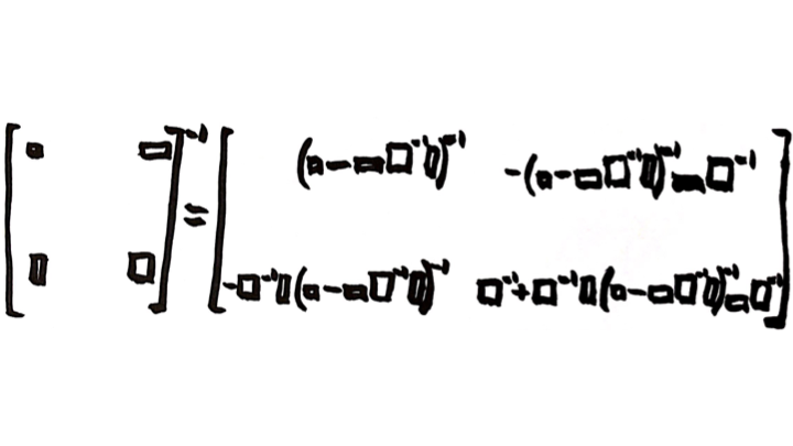
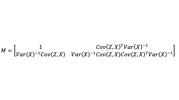
The Partitioned-Matrix Inversion Formula. This image first appeared in the the post “The Partitioned Matrix Inversion Formula.” Image created by Miles Spencer Kimball. I hereby give permission to use this image for anything whatsoever, as long as that use includes a link to this blog. For example, t-shirts with this picture (among other things) and supplysideliberal.com on them would be great! :) Here is a link to the Wikipedia article “Block Matrix,” which talks about the partitioned matrix inversion formula.
In “Eating Highly Processed Food is Correlated with Death” I observe:
In observational studies in epidemiology and the social sciences, variables that authors say have been “controlled for” are typically only partially controlled for. The reason is that almost all variables in epidemiological and social science data are measured with substantial error.
In the comments, someDude asks:
"If the coefficient of interest is knocked down substantially by partial controlling for a variable Z, it would be knocked down a lot more by fully controlling for a variable Z. "
Does this assume that the error is randomly distributed? If the error is biased (i.e. by a third underlying factor), I would think it could be the case that a "fully controlled Z" could either increase or decrease the the change in the coefficient of interest.
This post is meant to give a clear mathematical answer to that question. The answer, which I will back up in the rest of the post, is this:
Compare the coefficient estimates in a large-sample, ordinary-least-squares, multiple regression with (a) an accurately measured statistical control variable, (b) instead only that statistical control variable measured with error and (c) without the statistical control variable at all. Then all coefficient estimates with the statistical control variable measured with error (b) will be a weighted average of (a) the coefficient estimates with that statistical control variable measured accurately and (c) that statistical control variable excluded. The weight showing how far inclusion of the error-ridden statistical control variable moves the results toward what they would be with an accurate measure of that variable is equal to the fraction of signal in (signal + noise), where “signal” is the variance of the accurately measured control variable that is not explained by variables that were already in the regression, and “noise” is the variance of the measurement error.
To show this mathematically, define:
Y: dependent variable
X: vector of right-hand-side variables other than the control variable being added to the regression
Z: scalar control variable, accurately measured
v: scalar noise added to the control variable to get the observed proxy for the control variable. Assumed uncorrelated with X, Y and Z.
Then, as the sample size gets large:

Define the following notation for the part of the variance of Z and of the variance of Z+v that are orthogonal from X (that is, the parts that are unpredictable by X and so represents additional signal from Z that was not already contained in X, plus the variance of noise in the case of Z+v). One can call this “the unique variance of Z”:
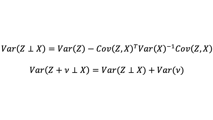
I put a reminder of the partitioned matrix inversion formula at the top of this post. Using that formula, and the fact that the unique variance of Z is a scalar, one finds:

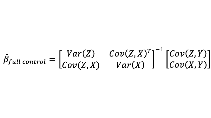
Defining
the OLS estimates are given by:
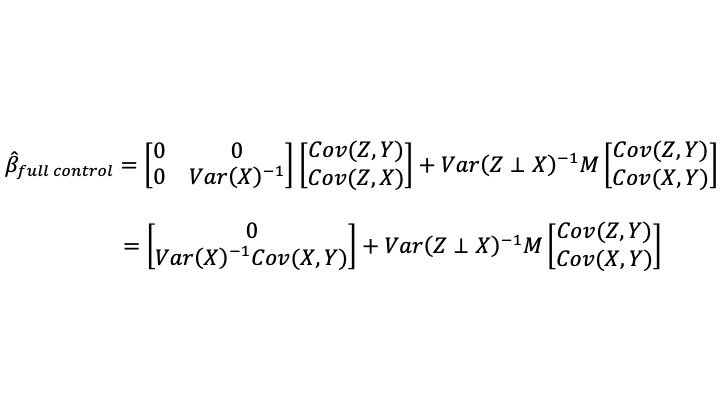
When only a noisy proxy for the statistical control variable is available (which is the situation 95% of the time), the formula becomes:
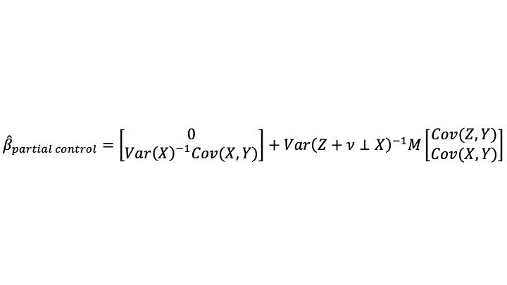
I claimed at the beginning of this post that the coefficients when using the noisy proxy for the statistical control variable were a weighted average of what one would get using only X on the right-hand side and what one would get using accurately measured data on Z. Note that what one would get using only X on the right-hand side of the equation is exactly what one would get in the limit as the variance of the noise added to Z (which is Var(v)) goes to infinity. So adding a very noisy proxy for Z is almost like leaving Z out of the equation entirely.
The weight can be interpreted from this equation:

As noted at the beginning of the post, the right notion of the signal variance is the unique variance of the accurately measured statistical control variable. The noise variance is exactly what one would expect: the variance of v.
I have established what I claimed at the beginning of the post.
Some readers may feel that the limitation of Z being a single scalar variable is a big limitation. It is worth noting that the results apply when adding many statistical control variables or their proxies, one at a time, sequentially. Beyond that, noncommutativity makes the problem more difficult: the commutativity of a scalar with the other matrices was important for the particular strategy used in the simplifications above.
Conclusion: Almost always, one has only a noisy proxy for a statistical control variable. Unless you use a measurement error model with this proxy you will not be controlling for the underlying statistical control variable. You will only be partially controlling for it. Even if you do not have enough information to fully identify the measurement error model you must think about that measurement error model and report a range of possible estimates based on different assumptions about the variance of the noise.
Remember that any departure from the absolutely correct theoretical construct can count as noise. For example, one might think one has a totally accurate measure of income, but income is really acting as a proxy for a broader range of household resources. In that case, income is a noisy proxy for the household resources that were the correct theoretical construct.
I strongly encourage everyone reading this to vigorously criticize any researcher who claims to be statistically controlling for something simply by putting a noisy proxy for that thing in a regression. This is wrong. Anyone doing it should be called out, so that we can get better statistical practice and get scientific activities to better serve our quest for the truth about how the world works.
Here are links to other posts that touch on statistical issues:
Let's Set Half a Percent as the Standard for Statistical Significance
Less Than 6 or More than 9 Hours of Sleep Signals a Higher Risk of Heart Attacks
Eggs May Be a Type of Food You Should Eat Sparingly, But Don't Blame Cholesterol Yet
Henry George Eloquently Makes the Case that Correlation Is Not Causation
The Carbohydrate-Insulin Model Wars

Writing on diet and health, I have been bemused to see the scientific heat that has raged over whether a lowcarb diet leads people to burn more calories, other things equal. It is an interesting question, because it speaks to whether in the energy balance equation
weight gain (in calorie equivalents) = calories in - calories out
the calories out are endogenous to what is eaten rather than simply being determined directly by conscious choices about how much to exercise.
My own view is that, in practice, the endogeneity of calories in to what is eaten is likely to be a much more powerful effect than the endogeneity of calories out to what is eaten. Metabolic ward studies are good at analyzing the endogeneity of calories out, but by their construction, abstract from any endogeneity of calories in that would occur in the wild by tightly controlling exactly what the subjects of the metabolic ward study eat.
The paper flagged at the top by David Ludwig, Paul Lakin, William Wong and Cara Ebeling is the latest salvo in an ongoing debate about a metabolic ward study done by folks associated with David Ludwig (including David himself). Much of the discussion is highly technical and difficult for an outsider to fully understand. But here is what I did manage to glean:
Much of the debate is arising because the sample sizes in this and similar experiments are too small. I feel the studies that have been done so far amply justify funding for larger experiments. I would be glad to give input on my opinions about how such experiments could be tweaked to deliver more powerful and more illuminating results.
One of the biggest technical issues beyond lower-than-optimal power involves how to control statistically for weight changes. Again, it is not so easy to fully understand all the issues with the time it is appropriate for me to devote to a single blog post, but I think weight changes need to be treated as an indicator of amount of fat burned with a large measurement error due to what I have called “mass-in/mass-out” effects. (See “Mass In/Mass Out: A Satire of Calories In/Calories Out.”) Whenever a right-hand-side variable is measured with error relative to the the exactly appropriate theoretical concept, a measurement error model is needed in order to get a consistent statistical estimate of the parameters of interest. I’ll write more (see “Adding a Variable Measured with Error to a Regression Only Partially Controls for that Variable”) about what happens when you try to control for something by using a variable afflicted with measurement error. (In brief, you will only be partially controlling for what you want to control for.)
David Ludwig, Paul Lakin, William Wong and Cara Ebeling are totally correct in specifying what one should focus on as the hypothesis of interest:
Hall et al. set a high bar for the Carbohydrate-Insulin Model by stating that “[p]roponents of low-carbohydrate diets have claimed that such diets result in a substantial increase in … [TEE] amounting to 400–600 kcal/day”. However, the original source for this assertion, Fein and Feinman [18], characterized this estimate as a “hypothesis that would need to be tested” based on extreme assumptions about gluconeogenesis, with the additional qualification that “we [do not] know the magnitude of the effect.” An estimate derived from experimental data—and one that would still hold major implications for obesity treatment if true—is in the range of 200 kcal/day [3]. At the same time, they set a low bar for themselves, citing a 6-day trial [16] (confounded by transient adaptive responses to macronutrient change [3]) and a nonrandomized pilot study [5] (confounded by weight loss [8]) as a basis for questioning DLW methodology. Elsewhere, Hall interpreted these studies as sufficient to “falsify” the Carbohydrate-Insulin Model [19]—but they do nothing of the kind. Indeed, a recent reanalysis of that pilot study suggests an effect similar to ours (≈250 kcal/day) [20].
Translated, this says that a 200-calorie-a-day difference is enough to be interesting. (Technically, the authors say “kilocalories,” but dieters always call kilocalories somewhat inaccurately by the nickname “calories.”) That should be obvious. For many people, 200 calories would be around 10% of the total calories they would consume and expend in a day. If a 200-calorie-a-day difference isn’t obvious beyond statistical noise, a metabolic ward study is definitely underpowered and needs a bigger sample!
Conclusion. In conclusion, let me emphasize again that the big issue with the worst carbs is that they make people hungry again relatively quickly, so that they eat more. (See “Forget Calorie Counting; It's the Insulin Index, Stupid” for which carbs are the worst.) Endogeneity of calories in might be a bigger deal than endogeneity of calories out. Moreover, because it is difficult for the body to switch back and forth between burning carbs and burning fat, a highcarb diet makes it painful to fast, while a lowcarb highfat diet when eating makes it relatively easy to fast. And fasting (substantial periods of time with no food, and only water or unsweetened coffee and tea as drinks) is powerful both for weight loss and many other good health-enhancing effects.
Update: David Ludwig comments on Twitter:
Perhaps: “endogeneity of calories in to what is eaten is likely to be a much more powerful effect than the endogeneity of calories out to what is eaten.” But the latter is a unique effect predicted by CIM. And if CIM is true, both arise from excess calorie storage in fat cells.
For annotated links to other posts on diet and health, see:
Here are some diet and health posts on authors involved in the Carbohydrate-Insulin Model Wars: