The Government and the Mob

I pitched this column to my editors as an Independence Day column. I am proud of our American experiment: attempting government of the people, by the people, and for the people. This column is about the principles behind that American experiment, from an economic perspective.
Calvin Coolidge on the Declaration of Independence

Thanks to the Wall Street Journal, I saw this passage from Calvin Coolidge’s “Address at the Celebration of the 150th Anniversary of the Declaration of Independence” in Philadelphia, July 5, 1926:
It was not because it was proposed to establish a new nation, but because it was proposed to establish a nation on new principles, that July 4, 1776, has come to be regarded as one of the greatest days in history. Great ideas do not burst upon the world unannounced. They are reached by a gradual development over a length of time usually proportionate to their importance. This is especially true of the principles laid down in the Declaration of Independence. Three very definite propositions were set out in its preamble regarding the nature of mankind and therefore of government. These were the doctrine that all men are created equal, that they are endowed with certain inalienable rights, and that therefore the source of the just powers of government must be derived from the consent of the governed.
If no one is to be accounted as born into a superior station, if there is to be no ruling class, and if all possess rights which can neither be bartered away nor taken from them by any earthly power, it follows as a matter of course that the practical authority of the Government has to rest on the consent of the governed. While these principles were not altogether new in political action, and were very far from new in political speculation, they had never been assembled before and declared in such a combination. But remarkable as this may be, it is not the chief distinction of the Declaration of Independence… .
It was the fact that our Declaration of Independence containing these immortal truths was the political action of a duly authorized and constituted representative public body in its sovereign capacity, supported by the force of general opinion and by the armies of Washington already in the field, which makes it the most important civil document in the world.
JP Koning: Does the Zero Lower Bound Exist Thanks to the Government's Paper Currency Monopoly?

I am grateful to JP Koning for agreeing to have this post from his blog Moneyness appear also as a guest post here on supplysideliberal.com. I tweeted “I love your post” and (lightly edited)
Your post “Does the zero lower bound exist thanks to the government’s paper currency monopoly” is very close to my answer in seminars of why private banks can’t undo what I propose central banks do.
For the record, I am not a fan of free banking. I am sympathetic with George Selgin’s claim (in a paper tweeted by David Beckworth) that the early days of central banking and 19th century US financial regulation may have been a step down in monetary stability and financial stability from free banking. But I believe that central banking with an electronic money system and monetary policy along the lines of what I discuss in my column “Optimal Monetary Policy: Could the Next Big Idea Come from the Blogosphere” is superior to free banking. I also give my view of the value of central banking in my post “Let’s Have an End to ‘End the Fed’” (Despite Ron Paul’s success in getting many people to chant “End the Fed” I think abolition of central banks and resumption of free banking is politically less likely–both in the US and in other nations–than the kind of electronic money system I recommend, so there is no strong argument for free banking as a politically easier solution to the zero lower bound problem.)
Many moons ago Matt Yglesias wrote that the “zero lower bound is a pure artifact of the existence of physical cash." In this post I’ll argue that the zero-lower bound, or ZLB, is an artifact of our modern central bank-managed monetary system, and not the existence of cash. In a free banking system in which private banks issue banknotes, competitive forces would force bankers to rapidly find ways to pierce below the ZLB, rendering the bound little more than a fleeting technicality.
What is the zero lower bound? When the economy’s expected rate of return drops significantly below 0%, interest rates charged by banks should follow into negative territory. But if banks set sub-zero interest rates on deposits, everyone will quickly convert them into central bank-issued paper currency. After all, why hold -2% yielding deposits when you can own 0% yielding cash? The inability to set negative interest rates is thezero-lower bound problem.
As I’ll illustrate, the threat of getting stuck at the zero-lower bound would impose such huge losses on private note-issuing banks that bank managers would quickly find creative ways to circumvent the problem. Central bankers, who aren’t beholden to the same financial motivations as private bankers, needn’t pursue these same zero-lower bound innovations with such zeal. This distinction has significant implications for the economy. Insofar as policies designed to remove the ZLB can prevent large macroeconomic distortions, central bankers are more likely to avoid such policies and destabilize the macroeconomy than private banker who, driven by bottom line concerns, will be quick to adopt ZLB-avoiding innovations.
Let’s set up our free banking system. Say that the Fed ceases issuing paper currency and only creates deposits. Into this void, private banks begin issuing their own paper dollar banknotes which can be exchanged for bank deposits at a rate of 1:1. This isn’t such a strange idea—for much of its history, Canada has enjoyed a privately-supplied paper currency. A few years later the economy nosedives and pessimism reigns. Private banks are desperate to decrease deposit rates into negative territory, say -4% or so. After all, banks earn income from the spread between the rate at which they borrow and the rate at which they invest. If, during bad times, a banker is investing at a -2% loss, he or she needs to be borrowing at -4% in order to earn spread income.
Unfortunately for our private banker, the intervening ZLB impedes rates from dropping into negative territory. Any attempt to cut to -4% and bank depositors will flock to convert negative yielding deposits into the bank’s 0% yielding banknotes. Very quickly the bank’s entire liability structure will be comprised of banknotes, a disastrous outcome since a bank that funds itself at 0% while investing at -2% will go broke very quick.
In a negative return world, profit-maximizing private banks would solve their ZLB problem using several strategies:
1. Remove Cash
If banks remove all of their already-issued cash from the economy in return for deposits, the deposits-to-cash escape route will be effectively erased, thereby clearing the way for banks to reduce deposit rates to -4%. One way to do this, courtesy of Bill Woolsey, would be for banks to issue cash with a call feature. Much like a convertible bond allows the bond issuer to force conversion upon investors, bank notes would carry a conversion clause permitting the issuing bank to call in all cash when it desires to reduce deposit rates below zero. [1]
2. Cease conversion into cash
Note-issuing banks might simply close the cash conversion window while allowing existing cash to remain in circulation. This would cut off any rush to convert deposits into cash upon a reduction of deposit rates to -4%. The price of existing cash would jump to a high enough level such that it would be expected to decline at a rate of 4% a year. Conversion stoppages are not without precedent. In 18th century Scotland, banks often issued notes with an option clause that allowed them to cease redemption should a bank run begin.
3. Penalize cash
By penalizing cash, a bank imposes a large enough cost on cash holders so that negative yielding deposits are no longer inferior to cash. There are plenty of ways for a bank to do this. One way is to impose a negative interest rate on cash by requiring cash holders to pay to "update” their bank notes lest they expire. This update fee, which would amount to around 4% a year, would forestall depositors from making a dash for cash when the bank sets deposit rates at -4%. In times past, locally-issued “scrip” like Worgl have had negative interest rates attached to them.
Another creative way for a banker to penalize cash is to impose a capital loss on cash holders. Rather than offering permanent 1:1 cash-to-deposit exchanges, banks might commit themselves to buying back cash (ie. redeeming it) in the future at an ever worsening rate to deposits. As long as the loss imposed on cash amounts to around 4% a year, depositors will not convert their deposits to cash en masse when deposit rates are cut to 4%.
In sum, a number of innovative routes are available for note-issuing banks to let their borrowing costs drop into negative territory. By necessity, private note-issuing banks will adopt these strategies in order to protect their shareholders from the painful effects of mass conversion of cheap deposit funding into relatively costly 0% cash.
That’s all fine and dandy, but our note-issuing mechanism is run by a centralized monopoly, not competing private banks. Because the ZLB is no less binding for central banks than it is for free banks, over the last few years economists and pundits have come up with all sorts of draconian techniques for central banks to escape the ZLB. There have been calls to ban cash, penalize it, and destroy it. At first I was somewhat appalled by these ideas as they seemed to be gross infringements on people’s ability to use cash. Over time I’ve realized that these authoritarian solutions are, somewhat paradoxically, the very same innovations that competing bankers would devise in a free banking world in order to free themselves of the ZLB problem. In other words, we can back out what a monopolist currency issuer *should* be doing to combat the ZLB by imagining what a network of competing banks *would* do. [2]
For instance, in a negative rate world a central bank ban on paper currency would be the equivalent of competing note-issuing banks simultaneously calling in their entire issue of paper currency in order to protect their solvency. If free banks were to penalize cash by redeeming it at ever deteriorating rates, this would be exactly the same strategy that Miles Kimball advocates central banks adopt in order to escape the ZLB.
That central banks have been so slow to evolve strategies for escaping from the ZLB could be due to any number of factors. Central banks aren’t privately owned nor are they disciplined by competition, and central bankers don’t have a mandate to turn a profit. Free banks, burdened by all of these checks, would be forced to rapidly adopt ZLB-escaping strategies or perish.
Further hampering efforts to get central banks like the Fed to innovate solutions to the ZLB is that these efforts might conflict with other goals. Withdrawing cash, penalizing it, or limiting conversion will put an end to, or at least diminish, the circulation of US paper dollars overseas. It might even result in the circulation of some other nation’s 0% yielding currency in the US. But the universal circulation of greenbacks is one of the most potent symbols of US hegemony, real or perceived. In the interests of protecting this symbol, innovations for escaping the ZLB may get short shrift. In a free banking system, these sorts of non-pecuniary motives are unlikely to outweigh the profit and loss calculation that dictates the necessity of adopting such innovations.
So the zero lower bound problem isn’t a problem with cash per se, it’s just a function of monopolistic intransigence. If you really want to short circuit the ZLB, better to devolve the provision of notes to profit-seeking private banks. Until then, hopefully evangelists like Miles Kimball succeed in getting central banks to adopt free banking-style contingency plans in preparation for the next time we experience a crisis that necessitates sub-zero interest rates.
[1] I confess that much of this post was inspired by ideas in two Bill Woolsey posts that I thought deserved wider circulation.
[2] The idea that harsh central bank policies like banning cash or penalizing currency might mimic free banking responses is a recurring theme on this blog. Here, I hypothesized that in a world characterized by free banking, legal tender laws might evolve naturally as the result of market choice. It’s a strange world.
Quartz #24—>After Crunching Reinhart and Rogoff's Data, We Found No Evidence High Debt Slows Growth

Here is the full text of my 24th Quartz column, that I coauthored with Yichuan Wang, “After crunching Reinhart and Rogoff’s data, we’ve concluded that high debt does not slow growth.” It is now brought home to supplysideliberal.com (and soon to Yichuan's Synthenomics). It was first published on May 29, 2013. Links to all my other columns can be found here. In particular, don’t miss the follow-up column “Examining the Entrails: Is There Any Evidence for an Effect of Debt on Growth in the Reinhart and Rogoff Data?”
If you want to mirror the content of this post on another site, that is possible for a limited time if you read the legal notice at this link and include both a link to the original Quartz column and the following copyright notice:
© May 29, 2013: Miles Kimball and Yichuan Wang, as first published on Quartz. Used by permission according to a temporary nonexclusive license expiring June 30, 2014. All rights reserved.
(Yichuan has agreed to extend permission on the same terms that I do.)
This column had a strong response. I have included the text of my companion column, with links to many of the responses after the text of the column itself. (For the comments attached to that companion post, you will still have to go to the original posting.) Other followup posts can be found in my “Short-Run Fiscal Policy” sub-blog.
Leaving aside monetary policy, the textbook Keynesian remedy for recession is to increase government spending or cut taxes. The obvious problem with that is that higher government spending and lower taxes tend to put the government deeper in debt. So the announcement on April 15, 2013 by University of Massachusetts at Amherst economists Thomas Herndon, Michael Ash and Robert Pollin that Carmen Reinhart and Ken Rogoff had made a mistake in their analysis claiming that debt leads to lower economic growth has been big news. Remarkably for a story so wonkish, the tale of Reinhart and Rogoff’s errors even made it onto the Colbert Report. Six weeks later, discussions of Herndon, Ash and Pollin’s challenge to Reinhart and Rogoff continue in earnest in the economics blogosphere, in the Wall Street Journal, and in the New York Times.
In defending the main conclusions of their work, while conceding some errors, Reinhart and Rogoff point out that even after the errors are corrected, there is a substantial negative correlation between debt levels and economic growth. That is a fair description of what Herndon, Ash and Pollin find, as discussed in an earlier Quartz column, “An Economist’s Mea Culpa: I relied on Reinhardt and Rogoff.” But, as mentioned there, and as Reinhart and Rogoff point out in their response to Herndon, Ash and Pollin, there is a key remaining issue of what causes what. It is well known among economists that low growth leads to extra debt because tax revenues go down and spending goes up in a recession. But does debt also cause low growth in a vicious cycle? That is the question.
We wanted to see for ourselves what Reinhart and Rogoff’s data could say about whether high national debt seems to cause low growth. In particular, we wanted to separate the effect of low growth in causing higher debt from any effect of higher debt in causing low growth. There is no way to do this perfectly. But we wanted to make the attempt. We had one key difference in our approach from many of the other analyses of Reinhart and Rogoff’s data: we decided to focus only on long-run effects. This is a way to avoid getting confused by the effects of business cycles such as the Great Recession that we are still recovering from. But one limitation of focusing on long-run effects is that it might leave out one of the more obvious problems with debt: the bond markets might at any time refuse to continue lending except at punitively high interest rates, causing debt crises like that have been faced by Greece, Ireland, and Cyprus, and to a lesser degree Spain and Italy. So far, debt crises like this have been rare for countries that have borrowed in their own currency, but are a serious danger for countries that borrow in a foreign currency or share a currency with many other countries in the euro zone.
Here is what we did to focus on long-run effects: to avoid being confused by business-cycle effects, we looked at the relationship between national debt and growth in the period of time from five to 10 years later. In their paper “Debt Overhangs, Past and Present,” Carmen Reinhart and Ken Rogoff, along with Vincent Reinhart, emphasize that most episodes of high national debt last a long time. That means that if high debt really causes low growth in a slow, corrosive way, we should be able to see high debt now associated with low growth far into the future for the simple reason that high debt now tends to be associated with high debt for quite some time into the future.
Here is the bottom line. Based on economic theory, it would be surprising indeed if high levels of national debt didn’t have at least some slow, corrosive negative effect on economic growth. And we still worry about the effects of debt. But the two of us could not find even a shred of evidence in the Reinhart and Rogoff data for a negative effect of government debt on growth.
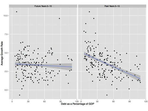
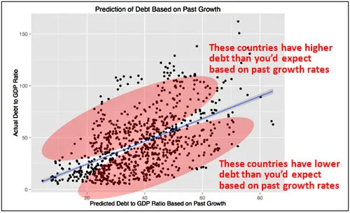
The graphs at the top show show our first take at analyzing the Reinhardt and Rogoff data. This first take seemed to indicate a large effect of low economic growth in the past in raising debt combined with a smaller, but still very important effect of high debt in lowering later economic growth. On the right panel of the graph above, you can see the strong downward slope that indicates a strong correlation between low growth rates in the period from ten years ago to five years ago with more debt, suggesting that low growth in the past causes high debt. On the left panel of the graph above, you can see the mild downward slope that indicates a weaker correlation between debt and lower growth in the period from five years later to ten years later, suggesting that debt might have some negative effect on growth in the long run. In order to avoid overstating the amount of data available, these graphs have only one dot for each five-year period in the data set. If our further analysis had confirmed these results, we were prepared to argue that the evidence suggested a serious worry about the effects of debt on growth. But the story the graphs above seem to tell dissolves on closer examination.
Given the strong effect past low growth seemed to have on debt, we felt that we needed to take into account the effect of past economic growth rates on debt more carefully when trying to tease out the effects in the other direction, of debt on later growth. Economists often use a technique called multiple regression analysis (or “ordinary least squares”) to take into account the effect of one thing when looking at the effect of something else. Here we are doing something that is quite close both in spirit and the numbers it generates for our analysis, but allows us to use graphs to show what is going on a little better.
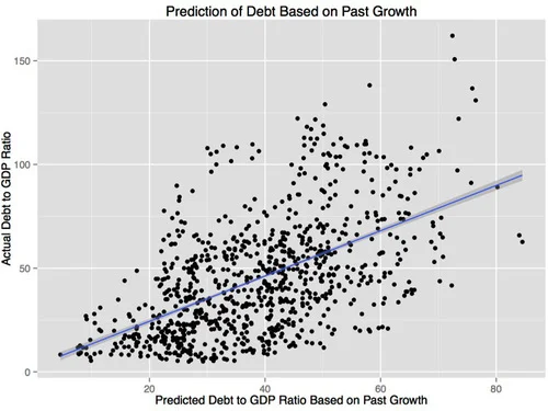
The effects of low economic growth in the past may not all come from business cycle effects. It is possible that there are political effects as well, in which a slowly growing pie to be divided makes it harder for different political factions to agree, resulting in deficits. Low growth in the past may also be a sign that a government is incompetent or dysfunctional in some other way that also causes high debt. So the way we took into account the effects of economic growth in the past on debt—and the effects on debt of the level of government competence that past growth may signify—was to look at what level of debt could be predicted by knowing the rates of economic growth from the past year, and in the three-year periods from 10 to 7 years ago, 7 to 4 years ago and 4 to 1 years ago. The graph below, labeled “Prediction of Debt Based on Past Growth” shows that knowing these various economic growth rates over the past 10 years helps a lot in predicting how high the ratio of national debt to GDP will be on a year by year basis. (Doing things on a year by year basis gives the best prediction, but means the graph has five times as many dots as the other scatter plots.) The “Prediction of Debt Based on Past Growth” graph shows that some countries, at some times, have debt above what one would expect based on past growth and some countries have debt below what one would expect based on past growth. If higher debt causes lower growth, then national debt beyond what could be predicted by past economic growth should be bad for future growth.
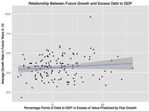
Our next graph below, labeled “Relationship Between Future Growth and Excess Debt to GDP” shows the relationship between a debt to GDP ratio beyond what would be predicted by past growth and economic growth 5 to 10 years later. Here there is no downward slope at all. In fact there is a small upward slope. This was surprising enough that we asked others we knew to see what they found when trying our basic approach. They bear no responsibility for our interpretation of the analysis here, but Owen Zidar, an economics graduate student at the University of California, Berkeley, and Daniel Weagley, graduate student in finance at the University of Michigan were generous enough to analyze the data from our angle to help alert us if they found we were dramatically off course and to suggest various ways to handle details. (In addition, Yu She, a student in the master’s of applied economics program at the University of Michigan proofread our computer code.) We have no doubt that someone could use a slightly different data set or tweak the analysis enough to make the small upward slope into a small downward slope. But the fact that we got a small upward slope so easily (on our first try with this approach of controlling for past growth more carefully) means that there is no robust evidence in the Reinhart and Rogoff data set for a negative long-run effect of debt on future growth once the effects of past growth on debt are taken into account. (We still get an upward slope when we do things on a year-by-year basis instead of looking at non-overlapping five-year growth periods.)
Daniel Weagley raised a very interesting issue that the very slight upward slope shown for the “Relationship Between Future Growth and Excess Debt to GDP” is composed of two different kinds of evidence. Times when countries in the data set, on average, have higher debt than would be predicted tend to be associated with higher growth in the period from five to 10 years later. But at any time, countries that have debt that is unexpectedly high not only compared to their own past growth, but also compared to the unexpected debt of other countries at that time, do indeed tend to have lower growth five to 10 years later. It is only speculating, but this is what one might expect if the main mechanism for long-run effects of debt on growth is more of the short-run effect we mentioned above: the danger that the “bond market vigilantes” will start demanding high interest rates. It is hard for the bond market vigilantes to take their money out of all government bonds everywhere in the world, so having debt that looks high compared to other countries at any given time might be what matters most.
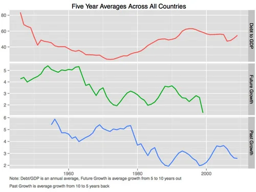
Our view is that evidence from trends in the average level of debt around the world over time are just as instructive as evidence from the cross-national evidence from debt in one country being higher than in other countries at a given time. Our last graph (just above) shows what the evidence from trends in average levels over time looks like. High debt levels in the late 1940s and the 1950s were followed five to 10 years later with relatively high growth. Low debt levels in the 1960s and 1970s were followed five to 10 years later by relatively low growth. High debt levels in the 1980s and 1990s were followed five to 10 years later by relatively high growth. If anyone can come up with a good argument for why this evidence from trends in the average levels over time should be dismissed, then only the cross-national evidence about debt in one country compared to another would remain, which by itself makes debt look bad for growth. But we argue that there is not enough justification to say that special occurrences each year make the evidence from trends in the average levels over time worthless. (Technically, we don’t think it is appropriate to use “year fixed effects” to soak up and throw away evidence from those trends over time in the average level of debt around the world.)
We don’t want anyone to take away the message that high levels of national debt are a matter of no concern. As discussed in “Why Austerity Budgets Won’t Save Your Economy,” the big problem with debt is that the only ways to avoid paying it back or paying interest on it forever are national bankruptcy or hyper-inflation. And unless the borrowed money is spent in ways that foster economic growth in a big way, paying it back or paying interest on it forever will mean future pain in the form of higher taxes or lower spending.
There is very little evidence that spending borrowed money on conventional Keynesian stimulus—spent in the ways dictated by what has become normal politics in the US, Europe and Japan—(or the kinds of tax cuts typically proposed) can stimulate the economy enough to avoid having to raise taxes or cut spending in the future to pay the debt back. There are three main ways to use debt to increase growth enough to avoid having to raise taxes or cut spending later:
1. Spending on national investments that have a very high return, such as in scientific research, fixing roads or bridges that have been sorely neglected.
2. Using government support to catalyze private borrowing by firms and households, such as government support for student loans, and temporary investment tax credits or Federal Lines of Credit to households used as a stimulus measure.
3. Issuing debt to create a sovereign wealth fund—that is, putting the money into the corporate stock and bond markets instead of spending it, as discussed in “Why the US needs its own sovereign wealth fund.” For anyone who thinks government debt is important as a form of collateral for private firms (see “How a US Sovereign Wealth Fund Can Alleviate a Scarcity of Safe Assets”), this is the way to get those benefits of debt, while earning more interest and dividends for tax payers than the extra debt costs. And a sovereign wealth fund (like breaking through the zero lower bound with electronic money) makes the tilt of governments toward short-term financing caused by current quantitative easing policies unnecessary.
But even if debt is used in ways that do require higher taxes or lower spending in the future, it may sometimes be worth it. If a country has its own currency, and borrows using appropriate long-term debt (so it only has to refinance a small fraction of the debt each year) the danger from bond market vigilantes can be kept to a minimum. And other than the danger from bond market vigilantes, we find no persuasive evidence from Reinhart and Rogoff’s data set to worry about anything but the higher future taxes or lower future spending needed to pay for that long-term debt. We look forward to further evidence and further thinking on the effects of debt. But our bottom line from this analysis, and the thinking we have been able to articulate above, is this: Done carefully, debt is not damning. Debt is just debt.
Companion Post
The title chosen by our editor is too strong, but not so much so that I objected to it; the title of this post is more accurate.
Yichuan only recently finished his first year at the University of Michigan. Yichuan’s blog is Synthenomics. You can see Yichuan on Twitter here. Let me say already that from reading Yichuan’s blog and working with him on this column, I know enough to strongly recommend Yichuan for admission to any Ph.D. program in economics in the world. He should finish has bachelor’s degree first, though.
I genuinely went into our analysis expecting to find evidence that high debt does cause low growth, though of course, to a much smaller extent than low growth causes high debt. I was fully prepared to argue (first to Yichuan and then to the world) that even a statistically insignificant negative effect of debt on growth that was plausibly causal had to be taken seriously from a Bayesian perspective. Our analysis set out the minimal hurdles I felt had to be jumped over to convince me that there was some solid evidence that high debt causes low growth. A key jump was not completed. That shifted my views.
I hope others will try to replicate our findings. That should let me rest easier.
From a theoretical point of view, I am especially intrigued by the possibility that any effect on growth from refinancing difficulties might depend on a country’s debt to GDP ratio compared to that of other countries. What I find remarkable is that despite the likely negative effect of debt on growth from refinancing difficulties, we found no overall negative effect of debt on growth. It is as if there is some other, positive effect of debt on growth to the extent a country’s relative debt position stays the same. Besides the obvious, but uncommonly realized, possibility of very wisely deployed deficit spending, I can think of two intriguing mechanisms that could generate such an effect. First, from a supply-side point of view, lower tax rates now could make growth look higher now, perhaps at the expense of growth at some future date when taxes have to be raised to pay off the debt, with interest. Second, government debt increases the supply of liquid (and often relatively safe) assets in the economy that can serve as good collateral. Any such effect could be achieved without creating a need for higher future taxes or lower future spending by investing the money raised in corporate stocks and bonds through a sovereign wealth fund.
I have thought a little about why borrowing in a currency one can print unilaterally makes such a difference to the reactions of the bond market to debt. One might think that the danger of repudiating the implied real debt repayment promises by inflation would mean the risks to bondholders for debt in one’s own currency would be almost the same as for debt in a foreign currency or a shared currency like the euro. But it is one thing to fear actual disappointing real repayment spread over some time and another thing to have to fear that the fear of other bondholders will cause a sudden inability of a government to make the next payment at all.
Note: Brad Delong writes:
Miles Kimball and Yichuan Wang confirm Arin Dube: Guest Post: Reinhart/Rogoff and Growth in a Time Before Debt | Next New Deal:

As I tweeted,
.@delong undersells our results. I would have read Arin Dube’s results alone as saying high debt *does* slow growth.
*Of course* low growth causes debt in a big way. But we need to know if high debt causes low growth, too. No ev it does!
In tweeting this, I mean,if I were convinced Arin Dube’s left graph were causal, the left graph seems to suggest that higher debt causes low growth in a very important way, though of course not in as big a way as slow growth causes higher debt. If it were causal, the left graph suggests it is the first 30% on the debt to GDP ratio that has the biggest effect on growth, not any 90% threshold. Yichuan and I are saying that the seeming effect of the first 30% on the debt to GDP ratio could be due in important measure to the effect of growth on debt, plus some serial correlation in growth rates. The nonlinearity could come from the fact that it takes quite high growth rates to keep a country from have some significant amounts of debt—as indicated by Arin Dube’s right graph, which is more likely to be primarily causal.
By the way, I should say that Yichuan and I had seen the Rortybomb piece on Arin Dube’s analysis, but we were not satisfied with it. But I want to give credit for this as a starting place for Yichuan and me in our thinking.
Brad Delong’s Reply: Thanks to Brad DeLong for posting the note above as part of his post “DeLong Smackdown Watch: Miles Kimball Says That Kimball and Wang is Much Stronger than Dube.”
Brad replies:
From my perspective, I tend to say that of course high debt causes low growth—if high debt makes people fearful, and leads to low equity valuations and high interest rates. The question is: what happens in the case of high debt when it comes accompanied by low interest rates and high equity values, whether on its own or via financial repression?
Thus I find Kimball and Wang’s results a little too strong on the high-debt-doesn’t-matter side for me to be entirely comfortable…
My Thoughts about What Brad Says in the Quote Just Above: As I noted above, my reaction is to what we Yichuan and I found is similar to Brad’s. There must be a negative effective of debt on growth through the bond vigilante channel, as Yichuan and I emphasize in our interpretation. For example, in our final paragraph, Yichuan and I write:
…other than the danger from bond market vigilantes, we find no persuasive evidence from Reinhart and Rogoff’s data set to worry about anything but the higher future taxes or lower future spending needed to pay for that long-term debt.
The surprise is the pattern that when countries around the world shifted toward higher debt than would be predicted by past growth, that later growth turned out to be somewhat higher than after countries around the world shifted to lower debt. It may be possible to explain why that evidence from trends in the average level of debt around the world over time should be dismissed, but if not, we should try to understand those time series patterns. It is hard to get definitive answers from the relatively small amount of evidence in macroeconomic time series, or even macroeconomic panels across countries, but given the importance of the issues, I think it is worth pondering the meaning of what limited evidence there is from trends in the average level of debt around the world over time. That is particularly true since in the current crisis, many people have, recommended precisely the kind of worldwide increase deficit spending—and therefore debt levels—that this limited evidence speaks to.
I am perfectly comfortable with the idea that the evidence from trends in the average level of debt around the world over time is limited enough so theoretical reasoning that shifts our priors could overwhelm the signal from the data. But I want to see that theoretical reasoning. And I would like to get reactions to my theoretical speculations above, about (1) supply-side benefits of lower taxes that reverse in sign in the future when the debt is paid for and (2) liquidity effects of government debt (which may also have a price later because of financial cycle dynamics).
Matt Yglesias’s Reaction: On MoneyBox, you can see Matthew Yglesias’s piece “After Running the Numbers Carefully There’s No Evidence that High Debt Levels Cause Slow Growth.” As I tweeted:
Don’t miss this excellent piece by @mattyglesias about my column with @yichuanw on debt and growth. Matt gets it.
In the preamble of my post bringing the full text of “An Economist’s Mea Culpa: I Relied on Reihnart and Rogoff" home to supplysideliberal.com, I write:
In terms of what Carmen Reinhart and Ken Rogoff should have done that they didn’t do, “Be very careful to double-check for mistakes” is obvious. But on consideration, I also felt dismayed that they didn’t do a bit more analysis on their data early on to make a rudimentary attempt to answer the question of causality. I wouldn’t have said it quite as strongly as Matthew Yglesias, but the sentiment is basically the same.
Paul Krugman’s Reaction: On his blog, Paul Krugman characterized our findings this way:
There is pretty good evidence that the relationship is not, in fact, causal, that low growth mainly causes high debt rather than the other way around.
Kevin Drum’s Reaction: On the Mother Jones blog, Kevin Drum gives a good take on our findings in his post “Debt Doesn’t Cause Low Growth. Low Growth Causes Low Growth.” He notices that we are not fans of debt. I like his version of one of our graphs:
Mark Gongloff’s Reaction: On Huffington Post, Mark Gongloff’s“Reinhart and Rogoff’s Pro-Austerity Research Now Even More Thoroughly Debunked by Studies” writes:
…University of Michigan economics professor Miles Kimball and University of Michigan undergraduate student Yichuan Wang write that they have crunched Reinhart and Rogoff’s data and found “not even a shred of evidence" that high debt levels lead to slower economic growth.
And a new paper by University of Massachusetts professor Arindrajit Dube finds evidence that Reinhart and Rogoff had the relationship between growth and debt backwards: Slow growth appears to cause higher debt, if anything….
This contradicts the conclusion of Reinhart and Rogoff’s 2010 paper, “Growth in a Time of Debt,” which has been used to justify austerity programs around the world. In that paper, and in many other papers, op-ed pieces and congressional testimony over the years, Reinhart And Rogoff have warned that high debt slows down growth, making it a huge problem to be dealt with immediately. The human costs of this error have been enormous….
At the same time, they have tried to distance themselves a bit from the chicken-and-egg problem of whether debt causes slow growth, or vice-versa. "The frontier question for research is the issue of causality,“ [Reinhart and Rogoff] said in their lengthy New York Times piece responding to Herndon. It looks like they should have thought a little harder about that frontier question three years ago.
There is an accompanying video by Zach Carter.
Paul Andrews Raises the Issue of Selection Bias: The most important response to our column that I have seen so far is Paul Andrews’s post "None the Wiser After Reinhart, Rogoff, et al.” This is the kind of response we were hoping for when we wrote “We look forward to further evidence and further thinking on the effects of debt.” Paul trenchantly points out the potential importance of selection bias:
What has not been highlighted though is that the Reinhart and Rogoff correlation as it stands now is potentially massively understated. Why? Due to selection bias, and the lack of a proper treatment of the nastiest effects of high debt: debt defaults and currency crises.
The Reinhart and Rogoff correlation is potentially artificially low due to selection bias. The core of their study focuses on 20 or so of the most healthy economies the world has ever seen. A random sampling of all economies would produce a more realistic correlation. Even this would entail a significant selection bias as there is likely to be a high correlation between countries who default on their debt and countries who fail to keep proper statistics.
Furthermore Reinhart and Rogoff’s study does not contain adjustments for debt defaults or currency crises. Any examples of debt defaults just show in the data as reductions in debt. So, if a country ran up massive debt, could’t pay it back, and defaulted, no problem! Debt goes to a lower figure, the ruinous effects of the run-up in debt is ignored. Any low growth ensuing from the default doesn’t look like it was caused by debt, because the debt no longer exists!
I think this issue needs to be taken very seriously. It would be a great public service for someone to put together the needed data set.
Note that Paul Andrews views are in line with our interpretation of our findings. Let me repeat our interpretation, with added emphasis:
…other than the danger from bond market vigilantes, we find no persuasive evidence from Reinhart and Rogoff’s data set to worry about anything but the higher future taxes or lower future spending needed to pay for that long-term debt.
Of course, it is disruptive to have a national bankruptcy. And national bankruptcies are more likely to happen at high levels of debt than low levels of debt (though other things matter as well, such as the efficiency of a nation’s tax system). And the fear by bondholders of a national bankruptcy can raise interest rates on government bonds in a way that can be very costly for a country. The key question for which the existing Reinhart and Rogoff data set is reasonably appropriate is the question of whether an advanced country has anything to fear from debt even if, for that particular country, no one ever seriously doubts that country will continue to pay on its debts.
Jessica Tozer: Boldly Going into a Future Where All Men and Women are Created Equal

In my sermons “UU Visions”“ and "So You Want to Save the World,” I say that a vision of how things should be is the starting place for trying to get there. Star Trek, along with entertainment, provides one such vision. The following is an excerpt from Jessica Tozer’s post “The Continuing Scientific Relevance of SciFi” written for the Armed with Science blog.
By the time Star Trek aired its first episode in 1966, Gene Roddenberry, the creator of Star Trek, was already a seasoned military veteran…. He flew planes in World War II, totaling 89 missions until he was honorably discharged at the rank of captain in 1945. During that time he saw people of all types in the military, pulling together for the sake of the mission, patriotism and each other. It was this social foundation upon which he built his future military premise.
“It speaks to some basic human needs that there is a tomorrow, that it’s not all going to be over in a big flash and a bomb, that the human race is improving, that we have things to be proud of as humans. No, ancient astronauts did not build the pyramids. Human beings built them because they’re clever and they work hard. Star Trek is about those things.” – Gene Roddenberry
… Roddenberry believed that the future would have evolved as much in science and technology as it would in social reform (miniskirts and beehives not withstanding).
“If man is to survive, he will have learned to take a delight in the essential differences between men and between cultures. He will learn that differences in ideas and attitudes are a delight, part of life’s exciting variety, not something to fear.” — Gene Roddenberry
Nichelle Nichols, who played Lt. Uhura (in TOS), often recalls the story about the time she was thinking of quitting Star Trek to return to Broadway, and how it was Martin Luther King, Jr. who talked her out of it. A fan of Star Trek, MLK Jr. mentioned to Nichelle that her show was one of the few he and his wife would allow their children to watch, and that she was a symbol for reform and change….
So she stayed. I mean, who could say no to that?
As a result, she would go on to film the episode “Plato’s Stepchildren”, the first example of a scripted inter-racial kiss between a white man and black woman on American television.
How’s that for social change?
It was a vision of successful racial integration. Men, women of all races working together as equals….
Whoopi Goldberg asked to have her role as Guinan on Star Trek TNG. She has been quoted as saying that she too, loved Star Trek as a kid, and that the show was the first indication that “black people make it to the future”. Geordi is blind and he flies a spaceship. Worf is an alien race that was once an enemy, serving proudly on the bridge of the Enterprise. Data is an android. I could go on and on.
Ariel Schwartz: Can Science Fiction Writers Inspire the World to Save Itself? →
The Hieroglyph project asks sci-fi writers to stop creating dark dystopias, and instead showed us visions of a better future, so that we work harder to get there.
John L. Davidson on Resolving the House Mystery: The Institutional Realities of House Construction

A Manufactured Home from Manufactured Home Source
John L. Davidson, is a Missouri lawyer who has an interesting blog, The Law of Drones, UAVs, UASs, and sUASs and is a frequent correspondent. You can find him on Twitter here. John had this intriguing response to my storify post "A House Mystery: Why Does House Construction Go Up in Booms and Down in Recessions?“ He was generous enough to agree to share this.
I have attached an article I wrote in 2005 for the South Carolina Bar which implicitly answers your questions. It has to do with banking law and LTV values.
Anyone in the housing or banking business should have give you an answer in 3 minutes. The answers collected in you series of tweets are wrong.
Understand that I have been representing homebuilders since 1980 and at one time represented one of the largest 10 private builders in the US.
While it may finally have changed with the Dobb Frank (law to new to know how it is being applied), before the latest Depression, there was no “equity or capital” in home building.
While nominally there was bank lending, in substance what we actually had was merchant banking with banks using construction loans to builders to give the appearance of lending, as I explain in my article.
This was accomplished by a manipulation of the LTV ratios. If you knew what you were doing, and had a good appraisal, a builder only needed 25% of the cost of the raw ground and could borrow all the rest. And by using “presales,” etc. the builder didn’t even need 25%.
In order to give the appearance of actually lending money, banks would monitor builders cash on hand and retained earnings. If a slow down appeared likely, banks would demand this cash be used to make greater down payments on renewal (home all LAC loans were 12 month, renewed in Sept., based on sales in spring and closings during summer).
My very large client failed in 1990 under this system. It was ironic. Its tax year was 8/31. It closed its tax year, making profits and paying income taxes. In September its lenders refused to renew loans unless all cash on hand was used to increase LTV ratios. The cash was paid and on 10/1 the firm failed. Since all lots and homes were subject to bank’s security interests, my client could not sell a home or lot and collect any money at a closing. The banks foreclosed and then found new builders, using same plans etc. to sell homes, when things picked up.
In economic substance, the developer was merely an employee of the bank, albeit the highest paid employee. The loan documents also gave the bank complete control over cash, who was paid, when, etc.
The bank acted to call for more cash merely for appearance sake for its regulators.
The entire system has nothing to do with interest rates, wages, material prices, etc. It was strictly a function of bank willingness to take risk. They could expand the inventory of homes or decrease such at any time. As they controlled all the lots—it takes 24 months, at best, to move from raw ground to finished lot and 30 months to a finished home—their actions controlled supply and prices.
Miles: Very interesting. But the question remains, why the banks don’t build more houses during the recession when it is cheaper to build houses?
John: Now that we have the right question, I have three or four answers, which kind of blend together to explain.
1)Banks do not make their money on the cost of the house. By law, they don’t share in profits. Banks make money on fees for loan origination and interest. Since they do not share in upside potential of build low, sell high, why take the risk?
2)Banks have minimal capital, so when economy dives and they have to take loan loss reserves, they don’t have capital to put into housing inventory.
3)Denial and appearances. Bankers do not think like merchant bankers. Lots of them think they are lenders. My good, look at denial elsewhere (even here in my one person law firm ;<) And, then you have what bankers think about all the time, What would the regulators think? If Bankers had financed new home construction in 2009 they could have been charged with bank fraud.
I am very serious on this point. The Bank fraud statute has been interpreted to make it a crime to make a “foolish” loan. Of course, true, when it comes to whether a loan is good or bad, is like art, in the eyes of the beholder. Read this case and consider whether if you represented a bank you would have told them to build homes in 2009?
In part the case says:
Reckless disregard equally satisfies the intent required under § 1344. See Willis v. United States, 87 F.3d 1004, 1007 (8th Cir.1996). What is charged in the indictment is not mere breach of the duty of a fiduciary to act honestly and prudently but a breach of that duty resulting in the reckless disposition of $2.7 million of Statebank funds. The defendants are adequately apprised of the charge of crimes committed in violation of § 1344(a).
We take the district court’s point that if the world price of oil had not fallen, all the troubles that befell the defendants might not have occurred. They might be today rich and respected citizens of Anchorage. They were unlucky in the extreme. Many financial irregularities come to light only in bad times. If the irregularities are criminal, as those charged here are portrayed as being, the defendants cannot excuse criminal conduct by the plea of bad luck.
4)No home equity of developers. I mentioned the LTV cash down issue. Well developers in fact never put any $$$ down. Most of the time the “cash” part of the LTV comes from a guaranty on a home (with equity) and a second mortgage. When homes sales drop, prices drop, available “equity” drops and capacity of banks to lend contracts. This was mentioned a lot by community banks, post 2008.
So, there you have it. A very detailed explanation about how the real world works.
Would appreciate you letting me know if you see any oversights in my thinking.
Data on Top Income Shares
This post is reblogged from isomorphismes:
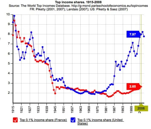
Incomes of the top .01%, 1915–2008 in France and United States
via @JWMason1
from the interactive The Top Incomes Database —
you can select countries such as Argentina, China, Indonesia, Ireland
and you can select upper quantiles like the lower half of the top percent; the .5%–.1%; top .1%; the top 10%–5%; and so on
and you can get income controls, price level indices, number of tax units, number of adults — the things you need to divide by in order to make apples-to-apples comparisons
Wooo, data!
Sticky Prices vs. Sticky Wages: A Debate Between Miles Kimball and Matthew Rognlie

Total Factor Productivity With and Without Utilization Adjustment Contrsucted by John Fernald Using Techniques from Susanto Basu’s, John Fernald’s and Miles Kimball’s paper “Are Technology Improvements Contractionary”
I had a very interesting email discussion with Matthew Rognlie (who blogs at mattrognlie.com) about price rigidity versus wage rigidity, sparked by my storify post “Why the Nominal GDP Target Should Go Up about 1% after a 1% Improvement in Technology,” where the argument hinges on whether prices are sticky, or wages are sticky, or both. The two of us decided to share our discussion with you.
Matthew:
I’m a grad student at MIT, and I’ve been enjoying your blog a great deal recently – it’s one of the only blogs I know for discussions of business cycle macro from someone with a really good grasp of modern work in the field. (Plus, I want to steal the “supply side liberal” label for myself.)
I was particularly interested to see your recent twitter discussion about price vs wage rigidity. My view is that there is extraordinarily strong evidence for nominal rigidities at the aggregate level – the most compelling being the old Mussa point about real exchange rate fluctuations under pegs vs. floating – but I am not so convinced that it comes from price rather than wage rigidity. In fact, recently I’ve been evolving toward the view that wage rigidity may be more important.
One of the difficulties in macro models of rigidity, I think, is that for reasons of analytical tractability most models tend to focus on one or two sources of rigidity, when in fact we have quite a few compelling candidates (the following categories are not precisely defined):
1. Nominal price rigidities: direct stickiness in nominal prices themselves, or perhaps (somewhat less plausibly in my view) stickiness in a nominal plan for prices, a la Mankiw and Reis.
2. Real price rigidities: various reasons why firms do not adjust prices so much in response to changes in marginal cost (possibly because there is some kind of strategic complementarity driven by the market structure, a la your 1995 aggregator), or why marginal costs themselves do not move much (aside from the obvious impact of wage rigidity, this could be due to the role of intermediates a la Basu).
3. Nominal wage rigidities: direct stickiness in nominal wages, either due to explicit contracts or implicit guarantees of wage stability, particularly in the downward direction. (Uncomfortable questions here about whether measured wages are really allocative, of course – I suspect their allocative role is surprisingly high.)
4. “Real" wage rigidities: either literal stickiness in inflation-adjusted wages a la Blanchard and Gali, or a set of frictions that prevent firms from adjusting wages as necessary, like the complexity of firms’ internal wage structure.
Anyway, my best guess is that all four of these are relevant, probably each to a substantial degree. Since these rigidities multiply, it’s easy to see how we could end up with a very high degree of aggregate nominal rigidity, to a degree that seems implausible when we’re scrutinizing a model with only one or two sources of rigidity.
I’m beginning to think that nominal wage rigidity, however, has a disproportionately important role, especially during recessions. There are many reasons why I think this, and I can’t list them all here, but the one I think is particularly interesting is the existence of nominal asymmetry. A large output gap is extraordinarily effective at bringing inflation down from, say, 8% to 2%, but far less effective at bringing about a drop from 2% to -2%. Even Japan, the prototypical example of a country in a prolonged deflationary slump, never saw a sustained rate below -1%. To me, the rapidity of disinflation compared to deflation suggests strong asymmetries in the nature of rigidity – and by far the most plausible candidate for asymmetry is nominal wage rigidity.
Certainly there are some other possible explanations as well. Perhaps inflation rates are very strongly influenced by forward-looking expectations of central bank policy – and while it’s plausible that a committed central bank might be trying to disinflate, no one would ever expect a central bank to actively attempt large-scale deflation. Or perhaps the much quicker rate of disinflation is due to higher nominal flexibility when the rate of inflation is further away from 0. Such alternatives are plausible, but my intuition is that quantitatively, it is very tough to explain the observed asymmetry without recourse to some asymmetry in the rigidity itself.
Another reason I am skeptical of the 80s-90s shift toward exclusively price-side rigidities is that I think some of the commonly stated arguments are not quite right. You mention in the twitter dialogue, for instance, that price rigidities justify a procyclical price level, while wage rigidities would lead to a countercyclical price level. While this is true to some extent, the procyclicality induced by sticky prices is much stronger than the countercyclicality induced by sticky wages. Indeed, in a benchmark model where labor is the only factor of production and there are no real shocks, the real wage under sticky wages is acyclical: it’s just the MPL divided by the markup, and when prices are flexible and firms can freely hit the desired markup, this is unaffected by nominal shocks. Countercyclicality under sticky wages only emerges due to flexibly priced factors of production other than labor.
My sense is that the countercyclicality induced by sticky wages is so weak that, if one introduces moderately sticky prices and market structure amplifying those sticky prices (i.e. a high intermediate share), it is easy to come out with a mildly procyclical real wage. And, indeed, cutting out oil shocks I’d say that the real wage has been just mildly procyclical in the postwar era – so this checks out. (Huang, Liu, and Phaneuf’s 2004 AER is a nice reference that works through some of this more explicitly.)
Anyway, I would love to have some more dialogue with you about the price vs. wage stickiness issue. I’ve been spending a fair amount of time recently thinking about ways to empirically distinguish between the two sources of rigidity, and I’ve also been talking to some of my fellow grad students - who seem to have pretty strong opinions in favor of wage rigidity. Maybe you can set my generation straight!
Miles:
My biggest objection to nominal wage rigidity is that observed wages are not allocative. It is hard to believe I would just give up on more labor input because the wage is high as opposed to asking my existing workers to work harder for the same pay, OR hire a worker at the high sticky wage level now (giving them a bigger piece of the pie of surplus from a match) and expecting them to understand that they might get a smaller piece of the pie of surplus from a match in the future. In other words, it makes no sense not to get more labor input just because you happen to have a high wage right now. I have no problem with wage rigidity when there is an actual union setting wages in the picture. But if the firm is a unilateral wage setter, and has a lot of influence over pace of work as well as wages, how can there be effective wage stickiness?
In other words, I don’t think it needs to be spelled out what is really going on inside the firm/worker relationship before we too readily agree that there are sticky wages. Unfortunately, most of the models there are either too rudimentary or too complex and focused on other issues to be of the help we would want in figuring out how effectively rigid wages are. I am just raising the skeptical point that if there is an allocative inefficiency from having the wrong amount of labor input, wouldn’t firms and workers together figure out some way around that? They have a long-term relationship in a way that few customer-supplier relationships can match.
A more simple prediction is that wages should look stickier the more conflict there is in the firm/worker relationship. Where firms and workers get along famously, there should be very little allocative inefficiency and therefore no allocative wage stickiness. Where firms and workers are at loggerheads, there could be a lot of effective wage stickiness.
One other point: one way in which nominal wage rigidity fails is that firms make workers contribute more for medical insurance. If you can cut benefits across the board in that way, and then have raises for some, you have loosened the downward nominal rigidity. Finally, don’t forget my point that the observation that technology improvements are contractionary can only work if there is substantial price stickiness. You can’t get that from wage stickiness alone. So that means price stickiness is a major factor in the economy–though there might also be wage stickiness.
My bottom line has been that if for tractability you have to choose between only price stickiness in a model and only wagestickiness, you are closer to reality with price stickiness. But if you can manage both and can deal with the micro issues of long-term labor relationships and variable effort, then it could be reasonable to have some wage stickiness too.
Matthew:
Thanks so much for your quick and detailed response. I apologize for my tardiness - I was working on a response Thursday night, but then things around here got a little crazy and I dropped it for a while.
I agree that the key issue is whether nominal wages indeed play an allocative role. (After all, there is plenty of evidence showing that the nominal wages themselves are remarkably sticky – this is uncontroversial enough that the key question is whether these payments are meaningful, or whether they’re installments in a long-term labor relationship.) And I have to concede that surely,wages are not allocative on a day-by-day basis: if I’m expected to come to work and do a good job every day, I don’t really care that I’m paid $100 on Mondays and $200 on Tuesdays. There is a deeply important sense in which labor relationships differ from spot markets, with incentives provided through long-term bargains rather than explicit transactions.
But I don’t think that the implicit contract between firm and worker is really so thorough. Instead, there are profound commitment and information failures that keep labor relationships far short of the first best. Here’s the most important data point in my view: firms lay off many workers during deep recessions with minimal severance pay. Surely if firms and workers could agree to anything ex ante, they would agree to avoid this: layoff during a recession is a deep blow with massive costs to career, wallet, and psyche. If firms were truly insuring their workers, they would need to fork over much more than a few weeks’ (or months’) pay; except in the lowest tier of jobs, unemployment insurance is not nearly enough to recover from the financial calamity of joblessness.
So intellectually, I agree with your puzzlement that firms and workers would fail to reach an arrangement flexible enough to avert the inefficiencies of wage rigidity. That’s missing some pretty low-hanging fruit! But when the ultimate low-hanging fruit is "don’t cast out large chunks of your workforce onto a brutal job market with only token assistance”, and we’re missing even that, I have to conclude that there are deep inefficiencies in labor relationships that economists do not fully understand. My guess is that commitment problems lead the contractual wage to play a surprisingly large allocative role. In normal times, the continuation surplus from the worker-employee match is enough to efficiently respond to small shocks; but when the benefit from defaulting on the worker-employee arrangement is large enough, firms do not hesitate to do so. And at that point, the allocative price is the contract wage, not the shadow price in a long-term efficient bargain.
Note that there is imperfect commitment on both sides of the relationship. In your hypothetical situation where a firm is happy to hire more workers at the market wage, but its internal wages are rigid and high, one possible solution is to bring in new workers at the high wage with an understanding that they will give up more of the surplus in the future. But workers’ lack of commitment prevents this: in the future, when they’re supposed to receive a below-market wage, they’ll simply jump ship.
This explains why firms are so reluctant to hire the long-term unemployed. To make up for the poor skills of an out-of-practice worker, they need to pay substantially less, but wage norms prevent them from doing so explicitly. (It’s totally conceivable to me that for the first 6 months, a long-term unemployed worker is only 50% as productive as an employed one. Firms might have some slack in setting entry wages, but most would never dream of paying worker A 50% as much as worker B for the same blue-collar job.) The obvious solution is to pay the new workers a decent salary coming in, under the tacit agreement that they’ll get less in the future to compensate their employers for rescuing them from unemployment. But again, these workers will simply renege on the agreement once they’re able – and this will be pretty easy for them, since their main obstacle on the job market was their joblessness, which has now been fixed.
I am just raising the skeptical point that if there is an allocative inefficiency from having the wrong amount of labor input, wouldn’t firms and workers together figure out some way around that? They have a long-term relationship in a way that few customer-supplier relationships can match.
I think that the comparison here to customer-supplier relationships is very interesting. I agree that at the retail level, customer-supplier pairs tend to be pretty fleeting – I do not have a long-term relationship with Walmart allowing us to pave over the inefficiencies resulting from sticky prices. Relationships higher on the input-output chart, on the other hand, often do last for long periods of time, possibly longer than most jobs. I don’t see why it should be any harder for Toyota to have an efficient long-term bargain with its suppliers than with its workers. And this is very problematic for the sticky price hypothesis, because stickiness at the retail level alone is just not enough. (As several pricing studies have documented, retail price stickiness and cyclicality have a strong negative correlation – many durable good prices are barely sticky at all, which is a huge problem given your results with Barsky and House.)
One other point: one way in which nominal wage rigidity fails is that firms make workers contribute more for medical insurance. If you can cut benefits across the board in that way, and then have raises for some, you have loosened the downward nominal rigidity.
This is a very interesting point, and I’ve heard several variations on it. (Health insurance premiums are the most important by far, but there are also 401(k) matches, etc.) This does indeed seem to be a way for firms to overcome, to a small extent, the norm against wage cuts. But I don’t think firms can get away with too much along this dimension – at most, they might manage to cut effective compensation by a few percentage points, and even this only if they’re in cyclical sectors. I am skeptical that this is enough to diminish the importance of nominal wage rigidity by very much, though of course it will become steadily more important as “fringe” benefits take up more and more of the compensation bundle.
Finally, don’t forget my point that the observation that technology improvements are contractionary can only work if there is substantial price stickiness. You can’t get that from wage stickiness alone. So that means price stickiness is a major factor in the economy–though there might also be wage stickiness.
I am a very, very, big admirer of your work on the purified residual with Basu and Fernald. I have to confess, though, that I give it a different interpretation. I have a strong prior that all “technology shocks” in the data, even when the Solow residual is carefully adjusted, are artifacts of the data – my experience doing empirical work tells me that there will always be residuals with no plausible structural interpretation. And from my admittedly amateurish understanding of technological change, I find it hard to believe that the stochastic process for productivity is really a random walk. Innovations diffuse much too slowly for that – instead, I’d model productivity as a two-dimensional stochastic process, where there are shocks to “technological knowledge”, but these shocks’ influence on productivity is spread out over a long period.
Bottom line: I don’t know what high-frequency variations in the purified Solow residual are really capturing, but whatever it is, I don’t think it has much to do with underlying technological progress. My skepticism owes a lot to the numbers themselves – I’m not sure what was happening in 2009 and 2010, but I didn’t see anything consistent with a huge technological boom in 2009 and then technological regress in 2010, as in the adjusted TFP series maintained by John Fernald. (One can go way back with this. Did TFP really decline in the year 2006? Did it decline for three consecutive quarters in 1996-97? Or for three consecutive quarters in 1994?)
Despite all this skepticism, though, I’m a huge fan of the work. But my interpretation of your results is “look, some meticulous and reasonable adjustments to TFP make the series look completely different, and give it completely different cyclical properties – so let’s be very careful drawing inferences from this stuff”, not “it turns out technology improvements are contractionary after all”. (Honestly, I think that meaningful high-frequency variation in TFP is basically something that Ed Prescott made up, so I’m not sure that “are technology shocks contractionary?” is even a well-posed question.) RBC had been cruising for far too long on basically spurious Solow residual estimates that ignored the overwhelming importance of factor utilization, and it was imperative that some smart macroeconomists do the legwork and show that this was untenable. I’m extremely glad you did, and I cite it whenever I get the chance. But I’m still not willing to treat the high-frequency shocks as structural, which is why I don’t view this as decisive in the sticky prices vs. wages debate.
A few years ago, I read an aside in Stiglitz’s Nobel autobiography that really shook me:
Economists spend enormous energy providing refined testing to their models. Economists often seem to forget that some of the most important theories in physics are either verified or refuted by a single observation, or a limited number of observations (e.g. Einstein’s theory of relativity, or the theory of black holes).
I really think that this is true: we often do very complicated, nontransparent estimation and testing of models, when in reality one or two carefully selected stylized facts could be much more decisive. My view is that the existence of mass layoffs during recessions with minimal severance, while perhaps not quite decisive, is one of these very important stylized facts - it appears to be a very important predictive failure of the implicit contract model.
Miles: Your point about the contractual wage being allocative for the layoff decision is well taken. But reduced hiring is at least as big a part of what makes the labor market what it is in recessions, and the contractual wage is not allocative at the hiring margin: those hired are just beginning an extended employment relationship. A model with stickywages at the layoff margin but effectively flexible wages at the hiring margin would be a very different model than one with sticky wages at both margins.
Let me defend the Basu, Fernald Kimball measurement of technology shocks. I agree that the blip up in the John Fernald’s series [the graph at the top] in 2009 is an artifact, but that was also a very unusual time and should not signal a big problem with the series at other times. The blip hints that hours and effort requirements went different ways during that episode, despite the theory that says an optimizing firm should move hours and the effort requirements they impose on workers (and the workweek of capital) in synch with each other. A reasonable theoretical explanation is that firms at that juncture put a premium on liquid funds. Putting a precautionary premium on liquid funds, they reduced their head count even below what demand warranted, and made remaining workers work harder in some many cases. This runs down worker good will, but in that crisis time, firms were willing to run down worker good will in order to protect their cash balances. The model treats firms as able to freely borrow and lend, and so omits any liquidity concerns on the part of firms, so it would not track that phenomenon.
On your theoretical doubt about the reasonableness of random walk technology, let me first say that a random walk for technology is much more plausible a priori than mean-reverting technology that implies that firms routinely backslide, as if they were forgetting technology. The random walk Susanto Basu, John Fernald and I find has very few negative technology shocks. At least at the annual level for the economy as a whole, technology shocks are mostly a matter of how much technology improves. (At the industry level, there are more negative technology shocks. To the extent these are not reflections of measurement error, we do not understand them very well.)
In general, I would like to see much more work done to find the stories behind the technology shocks that Susanto Basu, John Fernald and I find in the data. Because we compute the technology shocks at the industry or sectoral level, it should be possible to investigate where the shocks come from. Finding the story behind particular sectoral technology shocks in our data would be a very worthy topic for undergraduate theses, for example.
Let me talk about the gradual adoption of technology that you emphasize, given the little that we know now about economy-moving technology shocks. My view has been that technology shocks big enough to move the economy as a whole are a reflection of the steep part of the S-curve for technology adoption. The new technology is actually starting to spread long before we see it in the data. Then, there is a year when it goes from 15% adoption to 85% adoption, say, and that is the year we see the technology shock in the sectoral data, which then gets aggregated up to a macroeconomic technology shock. The standard errors are just to big to see clearly the gradual movement from 0 to 15% over several years or from 85% to almost 100% in several more years, but we can see the change in one year from 15% to 85%. What this means is that the technology shock in our data will be after, and predictable by, news reports of the new technology. At the Bank of Japan and to John Fernald at the San Francisco Fed, I have advocated that central banks should band together to do the staff work necessary to identify and predict macroeconomic technology shocks in advance, by gathering data on that initial introduction and adoption up to 15%. Hobbled as they are by the zero lower bound, central banks around the world have bigger problems to worry about right now, but in more halcyon times, better prediction of macroeconomic technology shocks would be a major part of their job. (In my column about Market Monetarism, NGDP targeting and optimal monetary policy, I talk both about how to eliminate the zero lower bound on nominal interest rates, and about how monetary policy can and should be adjusted for technology shocks.)
Matthew:
You said:
Your point about the contractual wage being allocative for the layoff decision is well taken. But reduced hiring is at least as big a part of what makes the labor market what it is in recessions, and the contractual wage is not allocative at the hiring margin: those hired are just beginning an extended employment relationship. A model with stickywages at the layoff margin but effectively flexible wages at the hiring margin would be a very different model than one with stickywages at both margins.
The same problems of imperfect commitment exist on the worker side. How can the effective wage for a new worker be much lower than the contractual wage? Only if the worker promises to compensate the employer by working at a below-market wage in the future. But it’s hard to make the worker keep his end of the implicit bargain – once he has other options, he’ll demand a fair, non-history-dependent wage. (Perhaps out of the loyalty to the firm for lifting him out of unemployment, he’ll be a little more pliable. Then again, he may be angry at having worse terms than his coworkers simply because he was unlucky enough to be hired during a recession.)
In general, my view of the employer-employee relationship is that it suffers from profound commitment and information failures. This is the only way to explain phenomena that couldn’t possibly be part of an efficient bargain - like layoffs in a depressed labor market. Most of the time, these failures are mitigated by the existence of surplus in the relationship between worker and firm. This surplus motivates both sides of the relationship to behave well in ways that can’t be codified in a formal contract. But when recession hits, at the contractual wage the surplus for the employer disappears, and it (inefficiently) terminates the relationship.
It’s similar for your hypothetical new worker. Suppose that he’s hired during a recession with the understanding that he’ll give up some of his future earnings. When the future arrives and prosperity returns, the worker won’t see any surplus from an ongoing relationship (other firms will compensate him fairly, without reference to the past), and he’ll terminate it. Any other outcome would be surprising. After all, apparently employers can’t commit to properly insure their workers against layoff, and if anything we’d expect implicit commitment to be easier for employers than workers.
In practice, neither side can reliably keep costly implicit promises, which means that the allocative wage can’t be too different from the contractual one. Wage stickiness matters on both margins.
Before continuing the debate on TFP, I want to take a step back and discuss the implications for wage rigidity. Initially, you mentioned that the apparent contractionary effect of technology shocks is evidence for price rather than wage rigidity. I took this as given and disputed the validity of measured TFP instead. But after further reflection I think that the former inference is equally problematic - even if the TFP series and impulse responses are flawless, we shouldn’t be so quick to settle on price stickiness.
Let’s take a look at Figure 4 from Basu, Fernald, Kimball (2006). Here, we see that after a 1% technology shock, the GDP deflator falls by 1% and the nominal wage stays almost exactly constant. Superficially, this seems much more consistent with sticky wages than sticky prices. That’s not completely fair, because maybe the measured wage isn’t allocative, and depending on the monetary rule there might be reasons why the price level eventually has to fall. (More on that in a second.)
But there are other problems with the story. The putative reason why technology improvements are contractionary is that the nominal money supply does not immediately adjust to the new level of output, which temporarily forces output below its natural level. (This is where the difference between sticky prices and wages comes in; with sticky wages alone, prices would fall to offset the increase in productivity, and there would be no pressure on the money supply.) In equilibrium, however, this all occurs via the impact of monetary policy on the real interest rate. If the path of the real interest rate doesn’t increase, monetary policy can’t be producing a contractionary outcome - at least not in this case. Yet this doesn’t seem to be happening in Figure 4, where the real fed funds rate has a negative impulse response.
More broadly, I don’t see why technology improvements should be contractionary in any model, at least with a realistic specification of the monetary policy rule. While it’s true that they are contractionary under a money supply or nominal GDP rule, monetary policy during the sample period generally didn’t operate according to such rules. (A possible, brief Volcker exception notwithstanding.) Instead, it’s probably best characterized as following some kind of interest rate rule, perhaps a Taylor rule with inertia. And in that case, technology shocks aren’t contractionary at all.
To explore this further, I fired up Dynare and calculated impulse responses to technology improvements in a basic New Keynesian model, under various combinations of assumptions. (Results are here: http://www.mit.edu/~mrognlie/tech_shock_results.pdf)
For monetary rules, I examined a basic Taylor rule, an inertial Taylor rule, and a money supply rule. In general, the shock was not contractionary for employment under either Taylor rule; this only happened for the money supply rule. In the case where a t=0 shock was anticipated at t=-1, there was generally a contraction in employment from t=-1 to t=0, which could conceivably produce the impulse responses in BFK. But this happened in a number of cases with wage rigidity too (albeit attenuated by the monetary reaction to a fall in inflation), so it’s not particularly strong evidence on the rigidity issue.
Furthermore, with an interest rate rule there was never a persistent decline in prices in response to the shock, except in the presence of wage rigidity. If we stipulate that the Fed followed an interest rate rule during the sample period, then the deflationary impact of a shock in Figure 4 is very powerful evidence for sticky wages.
All in all, it is difficult to reconcile the full set of impulse responses in BFK with any single model. But at the very least, the impulse responses provide just as much evidence for sticky wages as sticky prices. The only hint of sticky prices is the headline finding of a contraction – and the underlying story there is contradicted by the real interest rate decline in Figure 4.
[Administrative note: I’d like to mention the adjusted TFP series we discussed, but I’m not sure that we are using the same series. I was using the utilization-adjusted numbers from a spreadsheet on John Fernald’s website here: http://www.frbsf.org/csip/research/tfp/quarterly_tfp.xls It looks like this doesn’t actually implement all the corrections from your paper, so I don’t want to put too much emphasis on it. Notably, it looks like the utilization-adjusted TFP in his spreadsheet has just as frequent technological regress as regular TFP.]
My view has been that technology shocks big enough to move the economy as a whole are a reflection of the steep part of the S-curve for technology adoption. The new technology is actually starting to spread long before we see it in the data. Then, there is a year when it goes from 15% adoption to 85% adoption, say, and that is the year we see the technology shock in the sectoral data, which then gets aggregated up to a macroeconomic technology shock. The standard errors are just to big to see clearly the gradual movement from 0 to 15% over several years or from 85% to almost 100% in several more years, but we can see the change in one year from 15% to 85%.
I found this suggestion intriguing. I’d long had a vague intuition that micro-level technology improvements could not possibly produce a TFP series as erratic as the one we see in practice. But I hadn’t given this issue – in particular, the relationship between the S-curve of adoption and TFP growth at the macro level - nearly the same thought as you.
Rather than try to communicate my muddled intuition (which no one, including me, has good reason to trust), I decided to write a simple model to flesh out the relationship between the diffusion of micro-level technology improvements and the time series properties of aggregate productivity. The results are available here:
http://www.mit.edu/~mrognlie/tfp_micro_brief.pdf
I found that under fairly general assumptions, there is a remarkably straightforward connection between the pace of technology diffusion at the micro level and the autocorrelation of aggregate TFP growth. The autocorrelation implied by the model, however, turns out to be far higher than anything visible in the data.
In particular, using a logistic functional form, suppose we parameterize the diffusion curve such that it takes one year for a technology to go from 12% to 88% adoption. (Pretty fast!) Then the autocorrelation of TFP growth in consecutive quarters should be 0.91. At lags of two and three quarters, it should be 0.70 and 0.46. This contrasts markedly with the values in the actual data, which are near zero – regardless of whether we’re using standard TFP, adjusted TFP, labor productivity, etc.
With a slower – and in my view more realistic – pace of diffusion, the contrast between model and data becomes even more stark. Suppose now that it takes two years for a technology to go from 12% to 88%. Then the autocorrelation of growth at lags of 1, 2, and 3 quarters should be 0.98, 0.91, and 0.82. This is nothing like the data.
The underlying logic of the model is pretty straightforward. It says that if new technologies aren’t adopted instantaneously, but instead are spread smoothly over time, then aggregate TFP growth should inherit some of that smoothness. It shouldn’t be nearly uncorrelated from quarter to quarter, which is what we see in practice.
It’s possible that the difference between model and data is caused by measurement error. But it would have to be quite severe measurement error, and it’s a suspicious coincidence that the negative correlation induced by measurement error would be exactly enough to change near-1 correlations to near-0!
Regardless, I think this casts some doubt on any interpretation of TFP as the aggregate reflection of micro-level technological progress. And it only strengthens my longstanding suspicion that short-run variability in TFP is dominated by the effects of specification error.
Glenn Ellison's New Book: Hard Math for Elementary School

Glenn Ellison, the microeconomic theorist at MIT, has written a new book for kids who love math. Here is what Susan Athey had to say about it on her Facebook page, and gave me permission to post:
If your elementary school kids love math–this truly unique book is for you. There’s enough material in here to run a math club for two years, at least. It is really inspiring to see what happens when someone with deep love of math, an incredible gift for teaching, and years of experience with coaching kids in math teams and working with his three brilliant daughters comes up with when he puts his mind to it! Thanks so much for sharing what you’ve created with the rest of us, Glenn Ellison! (And I can’t believe you managed to get this done on top of everything else you are doing!)
My Ec 10 teacher Mary O'Keeffe also gave a rave review of the book on her math circle blog.
Susan pointed out that Glenn also has a book for older kids, Hard Math for Middle School.
Allison Schrager: The Economic Case for the US to Legalize All Drugs

Here is a link to Allison Schrager’s well-written and thoughtful column in favor of drug legalization. My reflections on her column below are not intended to be read on their own, but only after you have read Allison’s column.
I agree with Allison that we need to legalize the production and sale of drugs in order to take revenue, and therefore power, away from criminal gangs. But I think it is important that we do whatever we can to drive down the usage of dangerous drugs consistent with taking the drug trade out of the hands of criminals:
- Taxes on dangerous drugs as high as possible without encouraging large-scale smuggling;
- Age limits on drug purchases as strict as consistent with keeping the drug trade out of the hands of illegal gangs;
- Free drug treatment, financed by those taxes;
- Evidence-based public education campaigns against drug use, financed by those taxes;
- Demonization in the media and in polite company of those who (now legally) sell dangerous drugs;
- Mandatory, gruesome warnings like those we have for cigarettes;
- Widespread mandatory drug testing and penalties for use of dangerous drugs–but not for drug possession;
- Strict penalties for driving under the influence of drugs.
Notice that in order to keep the drug trade from going underground, prosecutors must not be allowed to use evidence that an individual purchased or possessed drugs as evidence that he or she used drugs. Evidence of use would have to come from some form of drug testing or from behavior.
Since drug use would still be illegal, social disapproval of drug use would still be encoded into law. But under this policy, any reemergence of illegal gangs selling drugs would be reason for a course correction liberalizing drug sales to an even greater degree.
Despite all the efforts I advocate above to discourage use of dangerous drugs, legalizing the production, sale and possession of drugs would have serious costs. Those costs have to be set against what I consider the even more serious costs of the drug war itself.
John Stuart Mill: A Remedy for the One-Sidedness of the Human Mind

I have often marvelled at how the subtle philosophy of great thinkers is reduced to a caricature by those who claim those thinkers as an inspiration. People are drawn to simplifications. And therein lies danger. John Stuart Mill writes about how that danger can be reduced by including in the intellectual ecosystem even those who are off-base in their judgments. The following is from On Liberty, Chapter II: “Of the Liberty of Thought and Discussion,” paragraphs 34 and 35:
It still remains to speak of one of the principal causes which make diversity of opinion advantageous, and will continue to do so until mankind shall have entered a stage of intellectual advancement which at present seems at an incalculable distance. We have hitherto considered only two possibilities: that the received opinion may be false, and some other opinion, consequently, true; or that, the received opinion being true, a conflict with the opposite error is essential to a clear apprehension and deep feeling of its truth. But there is a commoner case than either of these; when the conflicting doctrines, instead of being one true and the other false, share the truth between them; and the nonconforming opinion is needed to supply the remainder of the truth, of which the received doctrine embodies only a part. Popular opinions, on subjects not palpable to sense, are often true, but seldom or never the whole truth. They are a part of the truth; sometimes a greater, sometimes a smaller part, but exaggerated, distorted, and disjoined from the truths by which they ought to be accompanied and limited. Heretical opinions, on the other hand, are generally some of these suppressed and neglected truths, bursting the bonds which kept them down, and either seeking reconciliation with the truth contained in the common opinion, or fronting it as enemies, and setting themselves up, with similar exclusiveness, as the whole truth. The latter case is hitherto the most frequent, as, in the human mind, one-sidedness has always been the rule, and many-sidedness the exception. Hence, even in revolutions of opinion, one part of the truth usually sets while another rises. Even progress, which ought to superadd, for the most part only substitutes, one partial and incomplete truth for another; improvement consisting chiefly in this, that the new fragment of truth is more wanted, more adapted to the needs of the time, than that which it displaces. Such being the partial character of prevailing opinions, even when resting on a true foundation, every opinion which embodies somewhat of the portion of truth which the common opinion omits, ought to be considered precious, with whatever amount of error and confusion that truth may be blended. No sober judge of human affairs will feel bound to be indignant because those who force on our notice truths which we should otherwise have overlooked, overlook some of those which we see. Rather, he will think that so long as popular truth is one-sided, it is more desirable than otherwise that unpopular truth should have one-sided asserters too; such being usually the most energetic, and the most likely to compel reluctant attention to the fragment of wisdom which they proclaim as if it were the whole.
Thus, in the eighteenth century, when nearly all the instructed, and all those of the uninstructed who were led by them, were lost in admiration of what is called civilization, and of the marvels of modern science, literature, and philosophy, and while greatly overrating the amount of unlikeness between the men of modern and those of ancient times, indulged the belief that the whole of the difference was in their own favour; with what a salutary shock did the paradoxes of Rousseau explode like bombshells in the midst, dislocating the compact mass of one-sided opinion, and forcing its elements to recombine in a better form and with additional ingredients. Not that the current opinions were on the whole farther from the truth than Rousseau’s were; on the contrary, they were nearer to it; they contained more of positive truth, and very much less of error. Nevertheless there lay in Rousseau’s doctrine, and has floated down the stream of opinion along with it, a considerable amount of exactly those truths which the popular opinion wanted; and these are the deposit which was left behind when the flood subsided. The superior worth of simplicity of life, the enervating and demoralizing effect of the trammels and hypocrisies of artificial society, are ideas which have never been entirely absent from cultivated minds since Rousseau wrote; and they will in time produce their due effect, though at present needing to be asserted as much as ever, and to be asserted by deeds, for words, on this subject, have nearly exhausted their power.
Marlene King: Social Media + Pop Culture = ? →
I used a Google Chrome incognito window to try to make sure this is ungated. But let me know if you do find it is behind a paywall.
Jonah Berger: Going Viral

Like many other readers, I was fascinated by Richard Dawkins introduction of the idea of a meme in his book The Selfish Gene.

Wikipedia gives a good discussion of memes:
A meme (/ˈmiːm/; meem)[1] is “an idea, behavior, or style that spreads from person to person within a culture.”[2] A meme acts as a unit for carrying cultural ideas, symbols, or practices that can be transmitted from one mind to another through writing, speech, gestures, rituals, or other imitable phenomena. Supporters of the concept regard memes as cultural analogues to genes in that they self-replicate, mutate, and respond to selective pressures.[3]
The word meme is a shortening (modeled on gene) of mimeme (from Ancient Greek μίμημα Greek pronunciation: [míːmɛːma]mīmēma, “imitated thing”, from μιμεῖσθαι mimeisthai, “to imitate”, from μῖμος mimos "mime")[4] and it was coined by the British evolutionary biologist Richard Dawkins in The Selfish Gene (1976)[1][5] as a concept for discussion of evolutionary principles in explaining the spread of ideas and cultural phenomena. Examples of memes given in the book included melodies, catch-phrases, fashion, and the technology of building arches.[6]
Proponents theorize that memes may evolve by natural selection in a manner analogous to that of biological evolution. Memes do this through the processes of variation, mutation, competition, and inheritance, each of which influence a meme’s reproductive success. Memes spread through the behavior that they generate in their hosts. Memes that propagate less prolifically may become extinct, while others may survive, spread, and (for better or for worse) mutate. Memes that replicate most effectively enjoy more success, and some may replicate effectively even when they prove to be detrimental to the welfare of their hosts.[7]
A field of study called memetics[8] arose in the 1990s to explore the concepts and transmission of memes in terms of an evolutionary model.
Internet memes are a subset of memes in general. Wikipedia has a good discussion of this particular subset of memes as well:
An Internet meme may take the form of an image, hyperlink, video, picture, website, or hashtag. It may be just a word or phrase, including an intentional misspelling. These small movements tend to spread from person to person via social networks, blogs, direct email, or news sources. They may relate to various existing Internet cultures or subcultures, often created or spread on sites such as 4chan, Reddit and numerous others.
An Internet meme may stay the same or may evolve over time, by chance or through commentary, imitations, parody, or by incorporating news accounts about itself. Internet memes can evolve and spread extremely rapidly, sometimes reaching world-wide popularity within a few days. Internet memes usually are formed from some social interaction, pop culture reference, or situations people often find themselves in. Their rapid growth and impact has caught the attention of both researchers and industry.[3]Academically, researchers model how they evolve and predict which memes will survive and spread throughout the Web. Commercially, they are used in viral marketing where they are an inexpensive form of mass advertising.
But sometimes our image of an internet meme is too narrow. A tweet can easily become an internet meme if it is retweeted and modified. Thinking of bigger chunks of text, even a blog post sometimes both spreads in its original form and inspires other blog posts that can be considered mutated forms of the original blog post. And thinking just a bit smaller than a tweet, a link to a blog post can definitely be a meme, coevolving with different combinations of surrounding text recommending or denigrating what is at the link–sometimes just the surrounding text of a tweet and sometimes the surrounding text of an entire blog post that flags what is at the link. So those of us who care how many people read what we have to say have reason to be interested in the principles that determine when tweet, a post or a link will be contagious or not. In other words, what does it take to go viral?
Jonah Berger’s book Contagious gives answers based on research Jonah has done as a Marketing professor at the Wharton school. Jonah identifies six dimensions of a message that make it more likely to spread. Here are my notes what Jonah has to say about those six dimensions, for which Jonah gives the acronym STEPPS:
1. Social Currency: We share things that make us look good.
Jonah emphasizes three ways to make people want to share something in order to look good.
- Inner Remarkability: making clear how remarkable something is. Two examples of remarkabilility are the Snapple facts on the inside of Snapple lids and the video series “Will It Blend?” showing Blendtec blenders grinding up just about anything, the more entertaining the better. Note how what is remarkable about the Blendtec blenders is brought out and dramatized in a non-obvious and entertaining way.
- Leverage Game Mechanics: Make a good game out of being a fan. Here the allure of becoming the Foursquare mayor of some establishment is a great example.
- Make People Feel Like Insiders: Here, counterintuitively, creating a sense of scarcity, exclusivity, and the need for inside knowledge to access everything, can make something more attractive. Of course, if you can get away with the illusion of scarcity and exclusivity rather than the reality, more people can be brought on board.
2. Triggers: Top of mind, tip of tongue.
Here the key idea is to tie what you are trying to promote to some trigger that will happen often in someone’s environment.
- Budweiser’s “Wassup” campaign might seem uninspired, but it tied Budweiser beer to what was a common greeting at the time among a key demographic of young males.
- The “Kitkat and Coffee” campaign tied Kitkat chocolate bars to a very frequent occurrence in many people’s days: drinking coffee.
- The lines “Thinking about Dinner? Think About Boston Market” helped trigger thoughts of Boston Market at a time of day at which they hadn’t previously had as much business.
- The trigger can even be the communications of one’s adversary, as in the anti-smoking ads riffing off of the Marlboro Man commercials:

3. Emotion: When we care, we share.
The non-obvious finding here is that high arousal emotions such as
- awe (including the wonder of science)
- excitement
- amusement (humor)
- anger
- anxiety
–regardless of whether they are positive or negative–encourage sharing more than low arousal emotions such as contentment and sadness. Indeed, arousal is so important for sharing, experiments indicate that even the physiological arousal induced by making people run in place can cause people to share an article more often.
To find the emotional core of an idea, so that emotional core can be highlighted, Jonah endorses the technique of asking why you think people are doing something, then asking “why is that important” three times. Of course, this could also be seen as a way to try to get at the underlying utility function: utility functions are implemented in important measure by emotions.
Jonah recommends Google’s “Paris Love” campaign as an example of showing how to demonstrate that something seemingly prosaic, such as search, can connect to deeper concerns.
4. Public: Built to show, built to grow.
Here I like the story of how Steve Jobs and his marketing expert Ken Segall decided that making the Apple log on a laptop look right-side up to other people when the laptop is in use was more important than making it look right-side up to the user at the moment of figuring out which way to turn to laptop to open it up. Jonah points out how the way the color yellow made them stand out helped make Livestrong wristbands a thing in the days before Lance Armstrong was disgraced

and how the color white made ipod headphones more noticeable than black would have.

Jonah also makes interesting points about how talking about certain kinds of bad behavior, by making it seem everyone is doing it, can actually encourage bad behavior. Think of Nancy Reagan’s “Just Say No” antidrug campaign:

An alternative is to try to highlight the alternative, desired behavior.
5. Practical Value: News you can use.
This dimension is fairly straightforward. But Jonah gives this interesting example of a video about how to shuck corn for corn on the cob that went viral in an older demographic where not many things go viral. He also points to the impulse to share information of presumed practical value as part of the reason it is so hard to eradicate the scientifically discredited idea that vaccines cause autism.
6. Stories: Information travels under the guise of idle chatter.
Here, Jonah uses the example of the Trojan horse, which works well on many levels: the horse brought Greek warriors into Troy, and the story of the Trojan horse brings the idea “never trust your enemies, even if they seem friendly” deep into the soul. He points out just how much information is carried along by good stories.
But Jonah cautions that to make a story valuable, what you are trying to promote has to be integral to the story. Crashing the Olympics and doing a belly flop makes a good story, but the advertising on the break-in diver’s outfit was not central to the story and was soon forgotten. By contrast, for Panda brand Cheese, the Panda backing up the threat “Never say no to Panda” is a memorable part of the stories of Panda mayhem in the cheese commercials, and Dove products at least have an integral supporting role to play in Dove’s memorable Evolution commercial illustrating the extent to which much makeup and photoshopping are behind salient images of beauty in our environment.
Applied Memetics for the Economics Blogger
Here are a few thought about how to use Jonah’s insights in trying to make a mark in the blogosphere and tweetosphere.
1. Social Currency
Inner Remarkability: I find the effort to encapsulate the inner remarkability of each post or idea in a tweet an interesting intellectual challenge. One good way to practice this is a tip I learned from Bonnie Kavoussi: try to find the most interesting quotation from someone else’s post and put that quotation in your tweet. That will win you friends from the authors of the posts, earn you more Twitter followers (remember that the author of the post will have a strong urge to retweet if you are advertising herhis post well), and hone your skills for when you want to advertise your own posts on Twitter.
Leverage Game Mechanics: In the blogosphere and on Twitter, we are associating with peers. Much of what they want is similar to what w want–to be noticed, to get our points across, to get new ideas. So helping them to win their game is basically a matter of being a good friend or colleague. For example, championing people’s best work and being generous in giving credit will win points.
Make People Feel Like Insiders: When writing for on online magazine (Quartz in my case), it feels I need to write as if the readers are reading me for the first time. By contrast, a blog is tailor-made to make readers feel like insiders. So it is valuable to have an independent blog alongside any writing I do for an online magazine.
2. Triggers
A common piece of advice to young tenure-track assistant professors is to do enough of one thing to become known for that thing. This is consistent with Jonah’s advice about triggers. Having people think of you every time a particular topic comes up is a good way to make sure people think of you. That doesn’t mean you need to be a Johnny-one-note, but it does mean the danger of being seen as a Johnny-one-note is overrated. Remember that readers can easily get variety by diversifying their reading between you and other bloggers. So they will be fine even if your blog specializes to one particular niche, or a small set of niches.
On Twitter, one way to associate yourself with a particular trigger is to use a hashtag. In addition to the hashtag #ImmigrationTweetDay that Adam Ozimek, Noah Smith and I created for Immigration Tweet Day, I have made frequent use of the hashtag #emoney, and I created the hashtag #nakedausterity.
3. Emotion
Economists often want to come across as cool and rational. But many of the most successful bloggers have quite a bit of emotion in their posts and tweets. I think Noah Smith’s blog Noahpinion is a good example of this. Noahpinion delivers humor, indignation, awe, and even the sense of anxiety that comes from watching him attack and wondering how the object of his attack will respond.
One simple aid to getting an emotional kick that both Noah and I use is to put illustrations at the top of most of our blog posts. I think more blogs would benefit from putting well-chosen illustrations at the top of posts.
4. Public
The secret to making a blog more public is simple: Twitter. Everything on Twitter is public, and every interaction with someone who has followers you don’t is a chance for someone new to realize you exist. Of course, you need to be saying something that will make people want to follow you once they notice that you exist.
Facebook helps too. I post links to my blog posts on my Facebook wall and have friended many economists.
Finally, the dueling blog posts in an online debate tend to attract attention.
5. Practical Value
In “Top 25 All-Time Posts and All 22 Quartz Columns in Order of Popularity, as of May 5, 2013,” I point out the two posts that are slowly and steadily gaining on posts that were faster out of the block:
- The Logarithmic Harmony of Percent Changes and Growth Rates
- Three Goals for Ph.D. Courses in Economics.
I think the reason is practical value. Economists love to understand the economy, but they also have to teach school. They are glad for help and advice for that task.
6. Stories
Let me make the following argument:
- a large portion of our brains is devoted to trying to understand the people in our social network;
- so the author of a blog is much more memorable than a blog, and
- a memorable story about a blog is almost always coded in people’s brains as a memorable story about the author of the blog.
Thus, to make a good story for your blog, it is important to “let people in.” That is, it pays off to let people get to know you. The challenge is then to let people get to know you without making them think you are so “full of yourself” that they flee in disgust. Economists as a rule have a surprisingly high tolerance for arrogance in others. But if you want non-economists to stick with you, you might want to inject some notes of humility into what you write.
One simple way to let people get to know you without seeming arrogant is to highlight a range of other people you think highly of. The set of people you think highly of is very revealing of who you are. (Of course, the set of people you criticize and attack is also very revealing of who you are, but not in the same way.)
Summary
Jonah Berger’s book Contagious is one of the few books in my life where I got to the end and then immediately and eagerly went back to the beginning to read it all over again for the second time. (I can’t remember another one.) Of course, it is a relatively short book. But still, it took a combination of great stories, interesting research results, and practical value for me as a blogger to motivate me to read it twice in quick succession. I recommend it. And I would be interested in your thoughts about how to get a better chance of having blog posts and tweets go viral.
Further Reading
Jonah recommends two other books that with insights into what makes an idea successful:
- Malcolm Gladwell’s The Tipping Point: is a fantastic read. But while it is filled with entertaining stories, the science has come a long way since it was released over a decade ago.”
- Chip Heath and Dan Heath's Made to Stick: Why Some Ideas Survive and Others Die…although the Heaths’ book focuses on making ideas ‘stick’–getting people to remember them–it says less about how to make products and ideas spread, or getting people to pass them on.”

Quartz #23—>QE or Not QE: Even Economists Need Lessons in Quantitative Easing, Bernanke Style

Here is the full text of my 23d Quartz column, “QE or Not QE: Even Economists need lessons in quantitative easing, Bernanke style,” now brought home to supplysideliberal.com. It was first published on May 14, 2013. Links to all my other columns can be found here.
If you want to mirror the content of this post on another site, that is possible for a limited time if you read the legal notice at this link and include both a link to the original Quartz column and the following copyright notice:
© May 14, 2013: Miles Kimball, as first published on Quartz. Used by permission according to a temporary nonexclusive license expiring June 30, 2014. All rights reserved.
Martin Feldstein is an eminent economist. In addition to being a prolific researcher, he served as head of US president Ronald Reagan’s Council of Economic Advisors, and made the National Bureau of Economic Research (NBER) what it is today—an institution that Paul Krugman called “the old-boy network of economics made flesh.” (I am one of the many economists who belongs to the NBER.) But Feldstein was wrong when he wrote in the Wall Street Journal last week, “The time has come for the Fed to recognize that it cannot stimulate growth,” in an op-ed headlined “The Federal Reserve’s Policy Dead End: Quantitative easing hasn’t led to faster growth. A better recovery depends on the White House and Congress.”
“Quantitative easing” or “QE” is when a central bank buys long-term or risky assets instead of purchasing short-term safe assets. One possible spark for Feldstein’s tirade against quantitative easing was the Fed’s announcement on May 1 that it “is prepared to increase or reduce the pace of its purchases” of long-term government bonds and mortgage-backed securities depending on the economic situation. This contrasts with the Fed’s announcement on March 20 that had only pledged as if the Fed would either keep the rate of purchases the same or scale them back, depending on circumstances. Philadelphia Fed Chief Charles Plosser described this as the Fed trying “to remind everybody” that it “has a dial that can move either way.”
So the Fed sounds more ready to turn to QE when needed than it did before.
Feldstein’s argument boils down to saying, “The Fed has done a lot of QE, but we are still hurting, economically. Therefore, QE has failed.” But here he misunderstands the way QE works. The special nature of QE means that the headline dollar figures for quantitative easing overstate how big a hammer any given program of QE is. Once one adjusts for the optical illusion that the headline dollar figures create for QE, there is no reason to think QE has a different effect than one should have expected. To explain why, let me lay out again the logic of one of the very first posts on my blog, “Trillions and Trillions: Getting Used to Balance Sheet Monetary Policy.” In that post I responded to Stephen Williamson, who misunderstood QE (or “balance sheet monetary policy,” as I call it there) in a way similar to Martin Feldstein.
To understand QE, it helps to focus on interest rates rather than quantities of assets purchased. Regular monetary policy operates by lowering safe short-term interest rates, and so pulling down the whole structure of interest rates: short-term, long-term, safe and risky. The trouble is that there is one safe interest rate that can’t be pulled down without a substantial reform to our monetary system: the zero interest rate on paper currency. (See “E-Money: How Paper Currency is Holding the US Recovery Back.”) There is no problem pulling other short-term safe interest rates (say on overnight loans between banks or on 3-month Treasury bills) down to that level of zero, but trying to lower other short-term safe rates below zero would just cause people to keep piles of paper currency to take advantage of the current government guarantee that you can get a zero interest rate on paper currency, which is higher than a negative interest rate.
As long as the zero interest rate on paper currency is left in place by the way we handle paper currency, the Fed’s inability to lower safe, short-term interest rates much below zero means that beyond a certain point it can’t use regular monetary policy to stimulate the economy any more. Once the Fed has hit the “zero lower bound,” it has to get more creative. What quantitative easing does is to compress—that is, squish down—the degree to which long-term and risky interest rates are higher than safe, short-term interest rates. The degree to which one interest rate is above another is called a “spread.” So what quantitative easing does is to squish down spreads. Since all interest rates matter for economic activity, if safe short-term interest rates stay at about zero, while long-term and risky interest rates get pushed down closer to zero, it will stimulate the economy. When firms and households borrow, the markets treat their debt as risky. And firms and households often want to borrow long term. So reducing risky and long-term interest rates makes it less expensive to borrow to buy equipment, hire coders to write software, build a factory, or build a house.
Some of the confusion around quantitative easing comes from the fact that in the kind of economic models that come most naturally to economists, in which everyone in sight is making perfect, deeply-insightful decisions given their situation, and financial traders can easily borrow as much as they want to, quantitative easing would have no effect. In those “frictionless” models, financial traders would just do the opposite of whatever the Fed does with quantitative easing, and cancel out all the effects. But it is important to understand that in these frictionless models where quantitative easing gets cancelled out, it has no important effects. Because in the frictionless models quantitative easing gets canceled out, it doesn’t stimulate the economy. But because in the frictionless models quantitative easing gets cancelled out it has no important effects. In the world where quantitative easing does nothing, it also has no side effects and no dangers. Any possible dangers of quantitative easing only occur in a world where quantitative easing actually works to stimulate the economy!
Now it should not surprise anyone that the world we live in does have frictions. People in financial markets do not always make perfect, deeply-insightful decisions: they often do nothing when they should have done something, and something when they should have done nothing. And financial traders cannot always borrow as much as they want, for as long as they want, to execute their bets against the Fed, as Berkeley professor and prominent economics blogger Brad DeLong explains entertainingly and effectively in “Moby Ben, or, the Washington Super-Whale: Hedge Fundies, the Federal Reserve, and Bernanke-Hatred.” But there is an important message in the way quantitative easing gets canceled out in frictionless economic models. Even in the real world, large doses of quantitative easing are needed to get the job done, since real-world financial traders do manage to counteract some of the effects of quantitative easing as they go about their normal business of trying to make good returns. And “large doses” means Fed purchases of long-term government bonds and mortgage-backed bonds that run into trillions and trillions of dollars. (As I discuss in “Why the US Needs Its Own Sovereign Wealth Fund,” quantitative easing would be more powerful if it involved buying corporate stocks and bonds instead of only long-term government bonds and mortgage-backed bonds.) It would have been a good idea for the Fed to do two or three times as much quantitative easing as it did early on in the recession, though there are currently enough signs of economic revival that it is unclear how much bigger the appropriate dosage is now.
Does QE work? Most academic and central bank analyses argue that it does. (See for example, work by Arvind Krishnamurthy and Annette Vising-Jorgenson of Northwestern University, and work by Signe Krogstrup, Samuel Reynard and Barbara Sutter of the Swiss National Bank. ) But I am also impressed by the decline in the yen since people began to believe that Japan would undertake an aggressive new round of QE. One yen is an aluminum coin that can float on the surface tension of water. Since September, it has floated down from being worth 1.25 cents (US) to less than a penny now. Exchange rates respond to interest rates, so the large fall in the yen is a strong hint that QE is working for Japan, as I predicted it would when I advocated massive QE for Japan back in June 2012.
Sometimes friction is a negative thing—something that engineers fight with grease and ball bearings. But if you are walking on ice across a frozen river, the little bit of friction still there between your boots and the ice allow you to get to the other side. It takes a lot of doing, but quantitative easing uses what friction there is in financial markets to help get us past our economic troubles. The folks at the Fed are not perfect, but they know how quantitative easing works better than Martin Feldstein does. If we had to depend on the White House and Congress for economic recovery, we would be in deep, deep trouble. It is a good thing we have the Fed.