Comparative Statics in a Long-Run Model

In levels, the key equations are 

Y = F(K,L)

C = C(Y-T)

Y = C + I + G + NX

or equivalently,

Y-C-G  =  S  =  I + NX

The following variables are exogenous, determined outside the model:

  • K = exogenous capital stock
  • L = exogenous amount of labor
  • T = taxes net of transfers and net of interest payments by the government (= taxes - transfers - interest payments by the government)
  • G = government purchases

Each problem will specify any way in which these exogenous variables change.  

In addition, please assume:

  • technology is unchanging as well as exogenous
  • NX = 0 in a closed economy. This also implies ΔNX=0. Assume a closed economy from here on. 

The problems will not spell these assumptions out. Just assume NX = 0 and that technology is unchanging.

The endogenous variables are:

  • Y = GDP
  • C = consumption
  • I = investment
  • S = national saving

In change form, using "·" to signify multiplication, the key equations are:

ΔY = MPK · ΔK + MPL · ΔL

ΔC = MPC · (ΔY - ΔT)

ΔY - ΔC -ΔG  =  ΔS =  ΔI + ΔNX

Remember to assume ΔNX=0 because the economy is closed. In a closed economy, the last equation becomes:

ΔY - ΔC -ΔG = ΔS = ΔI

There are three local parameters (slopes) in these change-form equations:

  • MPK = marginal product of capital
  • MPL = marginal product of labor
  • MPC = marginal propensity to consume

The problems always specify these local parameters. In the problems, always solve the equations in this order:

  1. ΔY = MPK · ΔK + MPL · ΔL
  2. ΔC = MPC · (ΔY - ΔT)
  3. ΔY - ΔC -ΔG  =  ΔS  =  ΔI

The numbers below are for toy economies; they may not be particularly realistic. Your job is to fill in ΔY, ΔC, ΔS and ΔI. If you want to print out the exercise and the answer, the files for the pictures below are here (1 is questions, 2 is answers).

Questions:


Slide1.png


Answers:


Slide2.png

Cobb-Douglas with Constant Returns to Scale Exercise

Here, let me start with the same beginning as to the "Returns to Scale Exercise":

Let %ΔX be an overall measure of the change in inputs. If each input changes by the same percentage, this is always equal to that percentage change in each input. 

If different inputs change by different percentages, this is a weighted average of the percent changes in each different input. As long as the firm is minimizing costs, the weights will be equal to the share of costs coming from paying for each input:

  • s_K = share_K = RK/(RK+WL) is the cost share of capital (the share of the cost of capital rentals in total cost.)
  • s_L = share_L = WL/(RK+WL) is the cost share of labor (the share of the cost of the wages of labor in total cost.) 

My post "The Shape of Production: Charles Cobb's and Paul Douglas's Boon to Economics" talks about this more in the case of constant-returns-to-scale Cobb-Douglas.

Thus, the total input measure is 

%ΔX = share_K  %ΔK + share_L  %ΔL

(Just to be clear about the notation, share_K and %ΔK are multiplying each other, and so on.) When (a) the degree of returns to scale is equal to 1 ("constant returns to scale"), and (b) the measures of input and output changes include everything, then the measure of technological progress is simply

%ΔA = %ΔY - %ΔX

In words, the change in technology is equal to the percent change in output minus the percent change in inputs overall (%ΔX). Technology improvements can show up as more output for the same input OR less input for the same output. It is also a technology improvement if output increases more than inputs. Things will get more complicated when there are increasing returns to scale or other issues. But this is good for now.  

The percent change in outputs minus the percent change in inputs %ΔY - %ΔX is called total factor productivity growth. It is often treated as a measure of technological change. But total factor productivity growth %ΔY - %ΔX  (= %ΔY - share_K  %ΔK + share_L  %ΔL when the only inputs are capital and labor) is an imperfect measure of technological change when their are increasing returns to scale (that is, when the degree of returns to scale γ = AC/MC > 1) or when the measures of inputs and outputs used are not comprehensive. Stay tuned for more on that later on in the semester.

These equations are exact with Platonic percentage changes and Cobb-Douglas with Constant Returns to Scale. Perhaps surprisingly, these equations are also very good approximations for other Constant-Returns-to-Scale production functions even when they are not Cobb-Douglas. 

Your task is to fill in the missing Platonic percent change in each row. Here is the pdf file with the questions (the missing piece for a row) on one side and the answers on the other. And here are the questions just below, and the answers further below on this post:


Rule of 70 Exercise

A Platonic change of y% always corresponds to multiplying by exp(.01 y). Approximating ln(2) as if it were exactly .7, this means that a 70% Platonic change corresponds to multiplying by 2. A -70% Platonic change corresponds to multiplying by .5. A 140% Platonic change corresponds to multiplying by 4. In this exercise, you are asked to mark which range the multiplication factor is in for the Platonic percentage changes shown at the top. Please act as if ln(2) were exactly equal to .7 so that a 70% Platonic change is exactly a doubling. 

Notice that a 70% Platonic change is multiplying by 2, which in turn is a 100% Earthly percentage change. A -70% Platonic change is multiplying by .5, which is a -50% Earthly percentage change. One illustration of how Platonic changes can be more convenient that Earthly percentage changes is that a 70% Platonic change followed by a -70% Platonic change gets you back to where you started. But a 100% Earthly percentage change followed by a -100% Earthly percentage change gets you to zero. And a 50% Earthly percentage change followed by a -50% Earthly percentage change gets you a -25% overall Earthly percentage change. 

If you want the exercise as a pdf with the questions on one side and the answers on the other, here it is. Or here it is on this blog post: 

Answers are below.


Returns to Scale Exercise

Let %ΔX be an overall measure of the change in inputs. If each input changes by the same percentage, this is always equal to that percentage change in each input. 

If different inputs change by different percentages, this is a weighted average of the percent changes in each different input. As long as the firm is minimizing costs, the weights will be equal to the share of costs coming from paying for each input:

  • s_K = share_K = RK/(RK+WL) is the cost share of capital (the share of the cost of capital rentals in total cost.)
  • s_L = share_L = WL/(RK+WL) is the cost share of labor (the share of the cost of the wages of labor in total cost.) 

My post "The Shape of Production: Charles Cobb's and Paul Douglas's Boon to Economics" talks about this more in the case of constant-returns-to-scale Cobb-Douglas.

Given %ΔX the degree of returns to scale γ is defined by the equation:

%ΔY = γ %ΔX

if there is no change in technology.

γ = the degree of returns to scale

DON'T CONFUSE SMALL GREEK LETTER γ WITH Y OR y!

The other key equation that you need is 

γ = AC/MC

where 

AC = average cost

MC = marginal cost

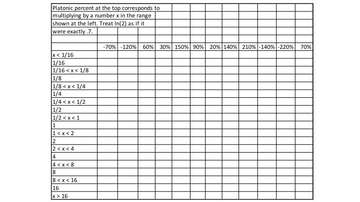
Your task in this exercise is to deduce the missing value in each row. One out of AC, MC, %ΔX and %ΔY is missing in each row of the questions. It is there in the answers. The degree of returns to scale γ is never explicitly stated in the row. But since each row assumes no change in technology, 

 γ = AC/MC =  %ΔY / %ΔX

Here is the way to show that  γ = AC/MC. Let C stand for total cost. (Sometimes we use C to stand for "consumption" but not here.) Then if Ω (the capital Greek letter Omega) is a price index for all the factors put together,   

MC = Ω ΔX / ΔY

AC = Ω X/Y

(The changes ΔX and ΔY in the definition of marginal cost stipulate that technology is not changing.) Since the Ω cancels,  

MC/AC = (ΔX/ΔY) / (X/Y)  =  (ΔX/X) / (ΔY/Y) ≈  %ΔX / %ΔY = 1/γ

AC/MC = (X/Y)  / (ΔX/ΔY)   =  (ΔY/Y) / (ΔX/X)  ≈   %ΔY / %ΔX =  γ

The only reason there is an approximation sign is that γ might not be constant. For small changes %ΔX and %ΔY, the degree of returns to scale γ will be approximately constant over the relevant range. For big changes it is some kind of complicated average γ over the relevant range that matters.

Why might γ not be constant? Here is an important case. Suppose there is a fixed cost FC and a constant marginal cost MC, then average cost AC will be declining from a very high level (essentially infinite for tiny amounts of output) toward MC. As the amount of output goes to infinity, the average cost AC converges to the constant marginal cost MC. This makes it clear that γ can't be constant in this case. 

You can either print out this one-sheet pdf file with the questions on one side and the answers on the other side, or you can look at the questions and later on the answers below in this post. Remember that these calculations all assume no change in technology


Student Guest Posts on supplysideliberal.com

Winter Semester, 2014

Winter Semester, 2015

Fall Semester, 2015

Winter Semester, 2016

University of Colorado Boulder, Spring Semester 2018

Supply and Demand: Elasticities and Comparative Statics

Before trying to do this exercise, be sure to read my post "The Logarithmic Harmony of Percent Changes and Growth Rates" and to study the section on prices elasticities of supply and demand in the "Growth Rates and Percent Changes" Powerpoint file (beginning on slide 21). The first key equation resulting from the algebra in that Powerpoint file is

(1)                       %ΔP = [%ΔD - %ΔS] / [η + ε]

The key notation here is

%ΔP = Platonic percent change in price = Δ ln(P)

%ΔQ = Platonic percent change in price = Δ ln(Q)

%ΔD = Platonic percent horizontal (quantity-metric) expansion of the demand curve.

%ΔS = Platonic percent horizontal (quantity-metric) expansion of the supply curve.

η = eta = price elasticity of supply (the slope of the supply curve when the horizontal axis is ln(Q) and the vertical axis is ln(P)).

ε= epsilon = price elasticity of demand (minus the slope of the demand curve when the horizontal axis is ln(Q) and the vertical axis is ln(P)). Note that for a normal downward sloping demand curve, this price elasticity of demand is expressed as a positive number. 

Now, let's solve for %ΔQ using 

%ΔQ = %ΔD - ε (%ΔP).

Substituting in %ΔP = [%ΔD - %ΔS] / [η + ε] yields

%ΔQ = %ΔD - (ε [%ΔD - %ΔS] / [η + ε]) = (η/[η + ε]) %ΔD + ( ε/[η + ε]) %ΔS

Try doing the same substitution into

%ΔQ = %ΔS + η (%ΔP)

You should get the very same answer, since the percent change in the equilibrium quantity must equal both the percent change in quantity demanded and the percent change in quantity supplied.  That is, 

(2)               %ΔQ = (η/[η + ε]) %ΔD + ( ε/[η + ε]) %ΔS

The demand and supply elasticities epsilon and eta are called "parameters." %ΔD and %ΔS are the exogenous changes. %ΔP and%ΔQ are the endogenous changes. Your task is to find the exogenous changes corresponding to the parameters and exogenous changes in each row of the table just below. Please look at the answers way below only after you have calculated all of your proposed answers.

Slide1.png


Here are the answers. Let me know if you think I have made an error in constructing the answer table.  

Slide2.png

%ΔQ = elasticity %ΔP; %Δ (PQ) = %ΔP+%ΔQ

The price elasticity of supply is defined as %ΔQ/%ΔP when moving along a supply curve. It is typically a positive number. (That is, supply curves slope up.)

The price elasticity of demand is defined as %ΔQ/%ΔP when moving along a demand curve. It is typically a negative number. Economists often talk about price elasticities of demand in terms of their absolute value, so that you have to supply the negative sign yourself from your general knowledge that increases in price reduce the quantity demanded. (That is, demand curves slope down.)

In the exercise below, the last four problems are more difficult, but for the rest, here is the procedure:

  1. Figure out whether the elasticity should have a negative sign because it is a demand elasticity or a positive sign because it is a supply elasticity. Together with the absolute value of the elasticity in the second column, that will give you the elasticity with a + or a - in the third column. 
  2. Multiply the (Platonic) percent change in the price by the elasticity to find the percent change in the quantity. 
  3. Add the percent change in the price and the percent change in the quantity to get the percent change in revenue PQ.  

Of the harder questions, some are missing %ΔP but have %ΔQ. All you need to do there is to divide %ΔQ by the signed elasticity to get %ΔP. Then you can add %ΔP to %ΔQ to get the percent change in PQ.  The last two questions are the hardest. There you need to do a bit of algebra:

%Δ (PQ) = (1 + elasticity) %ΔP

You can solve for %ΔP, and then multiply by the elasticity to get %ΔQ.

The answers are below as a filled-in table. 


elasticity pic 2.png

MV=PY, or equivalently %ΔM+%ΔV=%ΔP+%ΔY

This equation is called either “the Quantity Equation” or “the Equation of Exchange.” It is a very important equation for understanding the effects of money on the economy, but in this exercise, you can just treat the percent change version of the equation as a mathematical fact. Fill in the blank in each row and then check your answers. 

Note that if you divide each thing in the percent change version of the equation by time elapsed, you will get an equation in growth rates. The growth rate of the aggregate price index P is called inflation. Note also that if Divisia indices are used for money M (which is an aggregate of several different components), prices and quantities, then the percent change version of the equation is primary (most basic) and the MV=PY version would have to be deduced from the percent change version.