Monetary policy is far inside the production possibility frontier. We can do better. That is what I want to convince you of with this paper.
The worst danger we face in monetary policy during the next five years is complacency. I worry that central banks are patting themselves on the back because the world is finally crawling out of its business cycle hole. It is right to be grateful that things were not even worse in the aftermath of the Financial Crisis of 2008. But dangers abound, including (a) the likelihood that lesson that higher capital requirements are needed to avoid financial crises will be forgotten by key policy-makers, (b) the possibility of a dramatic collapse of Chinese real estate prices, and (c) the not-so-remote chance of a serious trade war.
A longer-term danger is that the rate of improvement in monetary policy will slow down as monetary policy researchers are drawn into simply justifying what central banks already happen to be doing. The assumption that people know what they are doing and are already following the best possible strategy may have an appropriate place in some areas of economics, but is especially inapt when applied to central banks. For one thing, the field of optimal monetary policy is very young, and its influence on central banks even more younger. For another, it is not easy to optimize in the face of complex political pressures and many self-interested actors eager to cloud one’s understanding with false worldviews.
Advances in monetary policy cannot come from armchair theorizing alone. trying ideas out is the only way to make a fully convincing case that they work—or don’t. But in general, the value of experimentation in public policy is underrated. Because central banks are usually in a good position to reverse something they try that doesn’t work, they are in an especially good position to do policy experiments for which a good argument can be made even if it is not 100 percent certain the experiment will be successful.
The Value of Interest Rate Rules
Because optimal monetary policy is still a work in progress, legislation that tied monetary policy to a specific rule would be a bad idea. But legislation requiring a central bank to choose some rule and to explain actions that deviate from that rule could be useful. To be precise, being required to choose a rule and explain deviations from it would be very helpful if the central bank did not hesitate to depart from the rule. Under this type of a rule, the emphasis is on the central bank explaining its actions. The point is not to directly constrain policy, but to force the central bank to approach monetary policy scientifically by noticing when it is departing from the rule it set itself and why.
So far, even without legislation, the Taylor Rule—essentially a description of the policy of the Fed under Volcker and Greenspan—has served this kind of useful function. Economists notice when the Fed departs from the Taylor Rule and talk about why.
The Taylor Rule has served another function: as a scaffolding for describing other words. Many important alternatives to the Taylor rule can readily be described as a modification of one of the Taylor Rule’s parameters or as the addition of an additional variable to the Taylor Rule.
In recent years, a shift toward purchasing assets other than short-term Treasury bills has complicated the specification of monetary policy. But Ricardo Reis, in his 2016 Jackson Hole presentation, argues that once the balance sheet is sufficiently large (about $1 trillion), it is again interest rates that matter after that. That is the perspective I take here.
What follows is, in effect, a research agenda for interest rate rules—a research agenda that will take many people to complete. The following sections discuss the following:
- eliminating the zero lower bound or any effective lower bound on interest rates
- tripling the coefficients in the Taylor rule
- reducing the penalty for changing directions
- reducing the presumption against moving more than 25 basis points at any given meeting
- a more equal balance between worrying about the output gap and worrying about fluctuations in inflation
- focusing on a price index that gives a greater weight to durables
- adjusting for risk premia
- pushing for strict enough leverage limits for financial firms that interest rate policy is freed up to focus on issues other than financial stability.
- having a nominal anchor.
Considering these possible developments in monetary policy is indeed only a research program, not a done deal. For each item individually, I have enough confidence research will ultimately vindicate it to be willing to state my views assertively. But though I don’t know which, it is likely that I have made some significant error in my thinking about at least one of the nine.
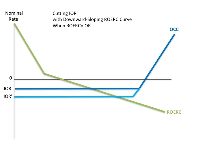
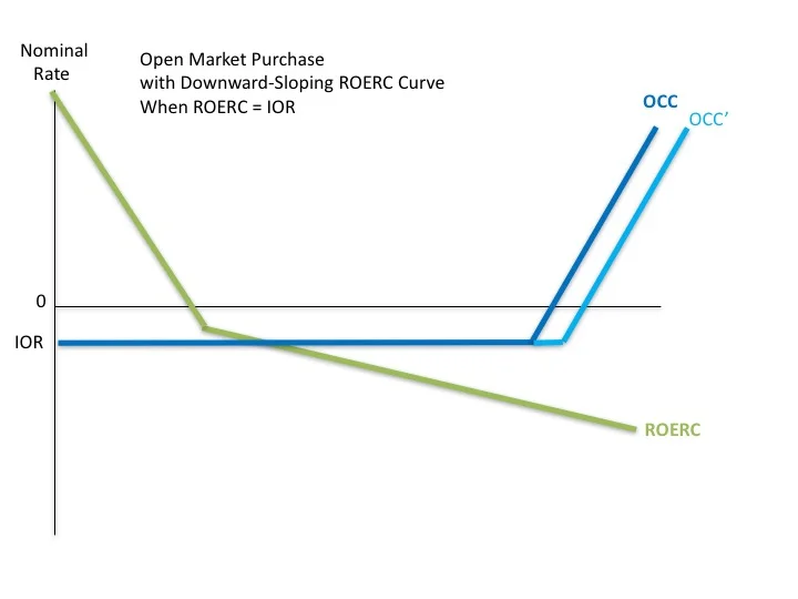
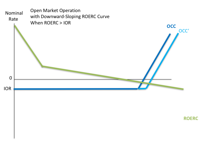
1. Eliminating the Zero Lower Bound and Any Effective Lower Bound for Nominal Rates
Eliminating any lower bound on interest rates is important for making sure that interest rate rules can get the job done in monetary policy. In “Negative Interest Rate Policy as Conventional Monetary Policy,” in the posts I flag in “How and Why to Eliminate the Zero Lower Bound: A Reader’s Guide” and with Ruchir Agarwal, in “Breaking Through the Zero Lower Bound,” I arguethat eliminating any lower bound on interest rates is quite feasible, both technically and politically. Although this has not happened yet, the attitude of central bankers and economists toward negative interest rates and towards the paper currency policies needed to eliminate any lower bound on interest rates have shifted remarkably in the last five years. “Negative Interest Rate Policy as Conventional Monetary Policy” gave this list of milestones for negative interest rate policy up to November 2015:
1. …. mild negative interest rates in the euro zone, Switzerland, Denmark and Sweden (see, for example, Randow, 2015).
2. The boldly titled 18 May, 2015 London conference on ‘Removing the Zero Lower Bound on Interest Rates’, cosponsored by Imperial College Business School, the Brevan Howard Centre for Financial Analysis, the Centre for Economic Policy Research and the Swiss National Bank.
3. The 19 May, 2015 Chief Economist’s Workshop at the Bank of England, which included keynote speeches by Ken Rogoff, presenting ‘Costs and Benefits to Phasing Out Paper Currency’ (Rogoff, 2014) and my presentation ‘18 Misconceptions about Eliminating the Zero Lower Bound’ (Kimball, 2015). …
4. Bank of England Chief Economist Andrew Haldane’s 18 September, 2015 speech, ‘How low can you go?’ (Haldane, 2015).
5. Ben Bernanke’s discussion of negative interest rate policy on his book tour (for Bernanke, 2015), ably reported by journalist Greg Robb in his Market Watch article ‘Fed officials seem ready to deploy negative rates in next crisis’ (Robb, 2015).
There have been at least four important milestones since then:
6. Narayana Kocherlakota’s advocacy of a robust negative interest rate policy. (See Kocherlakota, February 1, February 9, June 9 and September 1, 2016.)
7. The Brookings Institution’s June 6, 2016 conference “Negative interest rates: Lessons learned…so far” (video available at https://www.brookings.edu/events/negative-interest-rates-lessons-learned-so-far/ )
8. The publication of Ken Rogoff’s book, The Curse of Cash.
9. Marvin Goodfriend’s 2016 Jackson Hole talk “The Case for Unencumbering Interest Rate Policy at the Zero Bound” and other discussion of negative interest rate policy at that conference.
10. Ben Bernanke’s embrace of negative interest rates as a better alternative than raising the inflation target in his blog post “Modifying the Fed’s policy framework: Does a higher inflation target beat negative interest rates?”
In addition, I can testify to important shifts in attitudes based on the feedback from central bankers in presenting these ideas at central banks around the world since May 2013 and as recently as December 2016.[1] One objective indicator of this has been increased access by proponents of a robust negative interest rate policy to high-ranking central bank officials.
2. The Value of Large Movements in Interest Rates
Intuitively, the speed with which output gaps are closed and inflation fluctuations are stabilized depends is likely to depend on how dramatically a central bank is willing to move interest rates. It is notable that in explaining their monetary policy objectives, most central banks emphasize stabilizing inflation and unemployment, or stabilizing inflation alone.[2] But implicitly, many central banks act as if interest rate stabilization was also part of their mandates. This may be a mistake. The paper in this volume “The Yellen Rules” by Alex Nikolsko-Rzhevskyy, David H. Papell and Ruxandra Prodan provides suggestive evidence that increasing the size of the coefficients in the Taylor rule yields good outcomes; increasing the size of all the coefficients in the Taylor rule corresponds to increasing the size of interest rate movements. This is an idea that deserves much additional research.
For concreteness, let me talk about this as tripling the coefficients in the Taylor rule. Note that tripling the size of the coefficients in the Taylor rule only works on the downside if the lower bound on interest rates has been eliminated by changes in paper currency policy. Once the lower bound on interest rates has been eliminated, tripling the coefficients in the Taylor rule is likely to be a relatively safe experiment for a central bank to try.
3. Data Dependence in Both Directions
“Data dependence” has deservedly gained prominence as a central banking phrase. But in its current usage, “data dependence” of the action of a central bank at a given meeting almost always refers to incoming data determining either (a) whether the target interest rate will stay the same or go up in one part of the cycle, or (b) whether the target interest rate will stay the same or go down in another part of the cycle. Seldom does it refer to incoming data determining (c) whether the target interest rate stays the same, goes up or goes down. This is not the way formal models of optimal monetary policy work. If the target rate is where it should be at one meeting, there will be some optimal expected drift of the rate between that meeting and the next, but if meetings are relatively close together it would be strange if incoming news weren’t sometimes large enough to outweigh any such expected drift in the optimal policy. Indeed, if relevant news drove a diffusion process, the standard deviation of news would be proportional to the square root of the time gap between meetings, while the drift would be directly proportional to the time gap between meetings. Thus, when meetings are as close together as they are for most central banks (often as little as six weeks or one month), it would take quite large drift terms in the optimal policy to overcome the implications of news with such regularity that graphs of the target rate would take on the familiar stair-step pattern (going up the stairs, plateauing, then going down the stairs, and so on).
Indeed, I remember well a discussion with an economist at a foreign central bank in charge of calculating the implications of a formal optimal monetary policy rule. The rule had exactly the two-way character I am talking about, requiring the economist to add a fudge factor in order to get a one-way recommendation acceptable to the higher-ups.
One of the most important benefits of data dependence in both directions is that it allows more decisive movements in rates since it is considered easy to reverse course if later data suggests that move was too large. Indeed, the benchmark of optimal instrument theory with a quadratic loss function indicates that additive uncertainty does not affect the optimal level of the instrument. Thus, there is no need for a central bank that embraces “data dependence in both directions” to water down its reaction to a shock simply because it does not know what the future will bring. Staying put is more likely to be a big mistake than ignoring the uncertainty and going with the central bank’s best guess of the situation.
It is only when the effect size of the instrument itself is uncertain that movements in the instrument should be damped down. But one of the big advantages of interest rate policy—even negative interest rate policy—as compared to quantitative easing is that the size of the effect of a given movement in interest rates is much easier to judge given theory and experience than the effect of a given amount of long-term or risky asset purchases. Simple formal models predict that selling Treasury bills to buy long-term assets will have no effect, so any effect of quantitative easing is due to a nonstandard effect. Thus, any effect of such actions is due to one or more of many, many candidate nonstandard mechanisms. Theory then gives less guidance about the effects of quantitative easing than one might wish. And since the quantity of large scale asset purchases since 2008 was not enough to get economies quickly back on track, the relevant size of large scale asset purchases if one were to rely primarily on them in the next big recession is larger than anything for which we have experience. By contrast, in simple formal models, it is the real interest rate that matters for monetary policy. Monetary history provides a surprisingly large amount of experience with deep negative real rates. Other than paper currency problems that can be neutralized, only nonstandard mechanisms—such as institutional rigidities—would make low real rates coming from low nominal rates significantly different from low real rates coming from higher inflation.
One objection often made to “data dependence in both directions” is that reversing directions will make the central bank look bad—as if it doesn’t know what it is doing. A good way to deal with this communications problem is to spell out a formula in advance for how incoming data will determine the starting point for the monetary policy committee’s discussion of interest rates. Then it will be clear that it is the data itself that is reversing directions, not some central banker whim.
4. Stepping Away from Interest Rate Smoothing. The stair-step pattern of the target rate over time reflects not only an aversion to changing directions, but also an aversion to changing the interest rate too many basis points at any one meeting, where in the US the definition of “too many” is that traditionally, there is a substantial presumption against a movement of more than 25 basis points. The theoretical analogue of this behavior is often called “interest rate smoothing.”
There is a myth among many macroeconomists that commitment issues make it sensible to tie the current level of the target rate to the past level of the target rate with interest rate smoothing. Commitment issues can make the drift term in the optimal monetary policy rule stronger and thereby tilt things somewhat toward a predominant direction of movement, but it is hard to see how they would penalize large movements in the target rate at a given meeting of the monetary policy committee.
For “data dependence in both directions” and “stepping away from interest rate smoothing,” one need not embrace perfectly optimal monetary policy to get substantial improvements in monetary policy. Simply reducing the implicit penalty on changing directions or making a large movement in the target rate at a given meeting would bring benefits.
5. A More Equal Balance Between Output Stabilization and Inflation Stabilization
The Classical Dichotomy between real and nominal is akin to Descartes’ dichotomy between matter and mind. To break the mind-matter dichotomy, Descartes imagined that mind affected the body through the pineal gland (because it is one of the few parts of brain that does not come in a left-right pair). Where is the location analogous to the pineal gland where the Classical Dichotomy is broken in sticky price models? The actual markup of price over marginal cost (P/MC). For many sticky-price models, all the real part of the model needs to know is communicated by the actual markup (P/MC) acting as a sufficient statistic.[3] That is, if one takes as given the path of P/MC, one can often determine the behavior of all the relative prices and real quantities without knowing anything else about the monetary side of the model.
In cases where only one aggregate value for P/MC matters, the monetary model will differ from the real model it is built on top only in one dimension corresponding to the consequences of different values of P/MC. Thus, when duplicating the behavior of the underlying real model is attractive from the standpoint of welfare, all that is needed for excellent monetary policy is to choose the level of stimulus or reining in that yields the value of P/MC the underlying real model would have. Even when firm-level heterogeneity also matters for welfare, duplicating the aggregate behavior of the underlying real model is often an excellent monetary policy.
This logic is a big part of what lies behind the “divine coincidence” (Olivier Blanchard and Jordi Gali, 2007). That is, having, for many sticky-price models, only one dimension in which the vector of aggregate variables of the model can depart the vector of aggregate variables that would prevail in the underlying real model is a big part of the reason that the monetary policy that makes the output gap zero in those models also stabilizes inflation.
There are two main reasons the divine coincidence might fail. First, staying at the natural level of output generated by the underlying real model may not be the best feasible policy if there are fluctuations in the gap between the natural level of output and the ideal level of output (that would equate the social marginal benefit and social marginal cost of additional output).
Second, there may be more than one sectoral actual markup ratio P/MC that matters. Labor can be considered an intermediate good produced by its own sector far upstream, so sticky wages count as an additional sectoral price. But having sticky prices in the durables sector that follow a different path from sticky prices in the nondurables sector will also give the model more than one dimension in which it can depart from the underlying real model. The key to this second type of failure of the divine coincidence is fluctuations in the ratio between two different sticky-price aggregates.
When two aggregate markup ratios matter, it can be difficult for monetary policy to duplicate the behavior of the underlying real model. For monetary policy to keep the actual markups in two sectors simultaneously at the levels that would duplicate the behavior of the underlying real model even in the face of frequent shocks, monetary policy would have to be based on two instruments different enough in their effects that they could have a two-dimensional effect on the economy.
When the divine coincidence fails, there is a tradeoff between stabilizing output and stabilizing inflation. Then it becomes important to know how bad output gaps are compared to aggregate price fluctuations. Much of the cost of output gaps is quite intuitive: less smoothing of labor hours. The cost of departures from steady inflation are a little less intuitive: in formal models the main cost of price fluctuations is intensified leapfrogging of various firms’ prices over each other that can lead people to go to stores or to products that make no sense from an efficiency point of view. This cost of leapfrogging prices causing inefficient purchasing patterns is proportional to how responsive people are to prices. The higher the price elasticity of demand, the bigger the misallocations from the microeconomic price disturbances caused by leapfrogging prices when macroeconomic forces make aggregate prices to fluctuate.
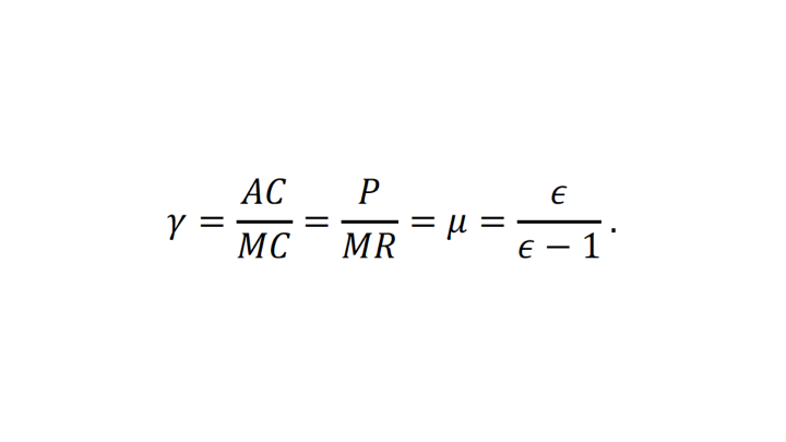
It is common in optimal monetary policy models to calibrate the price elasticity of demand at the firm level to a quite high value—often as high as 11. Where does this relatively high number come from? I have a suspicion. Susanto Basu and John Fernald (1996, 2002) and Basu (1997) estimate average returns to scale in the US economy of 1.1. Given free entry and exit of monopolistically competitive firms, in steady state average cost (AC) should equal price (P): if P > AC, there should be entry, while if P < AC there should be exit, leading to P=AC in steady state. Price adjustment makes marginal cost equal to marginal revenue in steady state. Thus, with free entry, in steady state,