Q&A: Why is Fiscal Policy So Close to Being Neutral in Many Modern Macro Models?

Q: Hi Miles: Sorry to bother you, but I’ve gotten hornswoggled into teaching macro again and there is one topic in kind of the evolution of macro that is eluding me.

And that question is, how did we get to fiscal policy irrelevance/ineffectiveness in the new keynesian dynamic model?

Is it a presumed Fed response to offset? Is it Ricardian Equivalence? Is it just that VARs show little response?

Can you give me a pointer about where to look?

A: This is something I teach in my graduate macro class. Fiscal policy irrelevance has nothing to do with sticky prices or not. It is all about investment. Without investment frictions, investment tends to be crowded out 1 for 1 by government purchases in both sticky-price and non-sticky-price models. (Let me ignore the effects on labor supply because of the impoverishment caused by higher G and also the opposite-direction effects of higher marginal taxes to pay for the higher G.) And that logic should extend to sticky wage models as well. Sticky prices don’t matter because aggregate demand doesn’t even go up. G up, I down.

Q-theory affects this in a different way than many people probably think. Q-theory is not really investment adjustment costs, it is investment smoothing, analogous to consumption smoothing. So it is totally forward looking. If a shock is going to last 4 or 5 years, then there is still fairly complete crowding out of investment

I think you will like my (unpublished) paper with Susanto Basu on investment planning costs. Here are its slides. (These are totally public.) But planning adjustment costs only let G stimulate the economy for 9 months are so (the same as the lag in the effect of monetary policy that comes from planning adjustment costs). I call that period of time the ultra-short run.

To the extent it seems that government purchases do have an affect on output longer than the ultra-short run, to me the leading candidates are:

  1. Monetary policy response. For example, when more military spending is needed as in Ramey and Shapiro, the central bank may be accomodative. This is speculative, I don’t know it to be true.
  2. Imperfect mobility of labor between production of capital and production of G. This is more credible in some areas than others. For example, building a government office building and a private office building should be doable by the same factors, so those shifts of factors between G and I should be easy. But the government has many other purchases of products of types that would be unusual in the private sector. 

If fiscal policy is about tax cuts to increase C, there are the usual permanent income issues plus the issue of how easily C can crowd out I. But consumption smoothing is likely much stronger than investment smoothing a la Q-theory, so that probably does work, as implicitly assumed in my paper “Getting the Biggest Bang for the Buck in Fiscal Policy” in arguing for the greater effectiveness of credit policy.  

Our Michigan PhD Chris Boehm has a paper on all of these issues that you should look at. 

One reason I call myself a Monetarist rather than a New Keynesian is because of these issues with fiscal policy. 

Helicopter Drops of Money Are Not the Answer

Among major news outlets with a print component, I am happy to say I have had occasion to praise negative interest rate reporting in the Wall Street Journal and in the Globe and Mail:

Unfortunately, Negative Interest Rate Reporting is Still in the Dark Ages at the Economist

The subtitle for the cover story for the February 20-26, 2016 Economist states their overall take quite clearly: 

“The World Economy: Out of ammo? Central bankers are running down their arsenal. But other options exist to stimulate the economy”

To give a further sense of that take on things, here are some key passages from that article:

One fear above all stalks the markets: that the rich world’s weapon against economic weakness no longer works. Ever since the crisis of 2007-08, the task of stimulating demand has fallen to central bankers. … 

… Despite central banks’ efforts, recoveries are still weak and inflation is low. Faith in monetary policy is wavering.

In this article, negative interest rates are dismissed with this one sentence:

Negative interest rates in Europe and Japan make investors worry about bank earnings, sending share prices lower.

(On negative interest rates and bank earnings, see my posts “How to Handle Worries about the Effect of Negative Interest Rates on Bank Profits with Two-Tiered Interest-on-Reserves Policies” and “If a Central Bank Cuts All of Its Interest Rates, Including the Paper Currency Interest Rate, Negative Interest Rates are a Much Fiercer Animal.”) 

The one other appearance of the word “negative” is in simply remarking

Borrowing has never been cheaper. Yields on more than $7 trillion of government bonds worldwide are now negative.

The Economist is wrong to dismiss negative interest rates. Indeed, I think the Economist will be unlikely to continue to dismiss negative interest rates as a powerful policy tool once one of their reporters takes the time to interview me, as they may sometime soon.

In the related article in the same issue, “Fighting the next recession: Unfamiliar ways forward–Policymakers in rich economies need to consider some radical approaches to tackling the next downturn,”the Economist says several negative things about negative rates without a change in paper currency policy, ignores the now well-heralded possibility of a negative paper currency interest rate (see how to deftly achieve a negative paper currency interest rate at the links in “How and Why to Eliminate the Zero Lower Bound: A Reader’s Guide”) and has this to say about negative interest rates with the alternative paper currency of abolishing paper currency:  

Since the existence of cash is a limit on how low interest rates can go, Andy Haldane, the chief economist of the Bank of England, and Ken Rogoff of Harvard University have proposed abolishing it altogether. But even if such radicalism were to prove feasible in a few countries, its effects might be limited. Savers would find alternative stores of value, such as precious metals or foreign banknotes, or pass on the cost of having money in the bank to others by making payments early.

The Economist, like John Cochrane (1, 2), is totally wrong about this. As my brother Chris and I point out in “However Low Interest Rates Might Go, the IRS Will Never Act Like a Bank,” it is almost impossible for anything but an unlimited opportunity to lend to the government at a zero interest rate to create a zero lower bound either or both because 

  1. most possible assets have a fluctuating price and therefore cannot provide a safe return, nor is there anything to prevent the price being big up high enough to generate a negative expected return, and

  2. all other opportunities to earn a zero interest rate in a negative interest rate environment would be exhausted long before investors had found a home for all of the assets they wanted a safe zero interest rate for.

And as for foreign assets, as I discuss in “Could the UK Be the First Country to Adopt Electronic Money?” the desire to purchase foreign assets when domestic assets are earning a negative return is part of the transmission mechanism, since it induces capital flows that in turn generate additional net exports. This is a feature of negative interest rate policy, not a bug. And in any case, it is not a concern for the world as a whole, to the extent the world as a whole turns to negative interest rates. 

The Economist Turns to Fiscal Policy

Instead of monetary policy, the Economist looks in important measure to some form of fiscal policy to provide economic stimulus, writing

The good news is that more can be done to jolt economies from their low-growth, low-inflation torpor (see Briefing). Plenty of policies are left, and all can pack a punch. The bad news is that central banks will need help from governments. Until now, central bankers have had to do the heavy lifting because politicians have been shamefully reluctant to share the burden. At least some of them have failed to grasp the need to have fiscal and monetary policy operating in concert. Indeed, many governments actively worked against monetary stimulus by embracing austerity. 

I am not so positive about fiscal policy. In “Narayana Kocherlakota Advocates Negative Rates and Criticizes the Conduct of US Fiscal Policy,” conscious of the power of deep negative interest rates to stimulate the economy, I write:

I tend to think that monetary policy should be used to stabilize the economy, not fiscal policy. Once monetary policy does its job, if the medium-run natural rate of interest is still low, then we should undertake more government investment. (See “The Medium-Run Natural Interest Rate and the Short-Run Natural Interest Rate.”) And we should undertake crucial government investments even if interest rates are high after the economy recovers. But it is just too hard to time government investment effectively in order to stabilize the economy.

Monetary policy has a lag of 6 to 12 months in its effects. Even so, it is much nimbler than government investment. Private investment and imports and exports can’t turn on a dime; hence the 6 to 12 month delay in the effect of monetary policy. But government investment typical takes even longer than that to turn around.

Using monetary policy as it should be used, aggregate demand is no longer scarce. Monetary policy can provide all the firepower needed.

Why Helicopter Drops Big Enough to Make People Think that the Government Will Go Bankrupt Unless There is Massive Inflation are Not the Answer

The Economist has a long list of policy prescriptions, among which using deep negative interest rates (combined with an appropriate paper currency policy) is conspicuously missing. But among all of the policy prescriptions, a helicopter drop of money takes pride of place as the first to get a full paragraph treatment:

The time has come for politicians to join the fight alongside central bankers. The most radical policy ideas fuse fiscal and monetary policy. One such option is to finance public spending (or tax cuts) directly by printing money—known as a “helicopter drop”. Unlike QE, a helicopter drop bypasses banks and financial markets, and puts freshly printed cash straight into people’s pockets. The sheer recklessness of this would, in theory, encourage people to spend the windfall, not save it.

The Economist discusses a helicopter drop further in the related article “Fighting the next recession: Unfamiliar ways forward–Policymakers in rich economies need to consider some radical approaches to tackling the next downturn”:

One way to raise expectations of inflation and boost aggregate demand is for a central bank and its finance ministry to collude in printing money to pay for public spending (or tax cuts). Such shenanigans are not possible in the euro zone, where the ECB is forbidden by treaty from buying government bonds directly. Elsewhere they might work as follows: the government announces a tax rebate and issues bonds to finance it, but instead of selling them to private investors swaps them for a deposit with the central bank. The central bank proceeds to cancel the bonds, and the government withdraws the money it has on deposit and gives it to citizens. “Helicopter money” of this sort—named in honour of a parable told by Milton Friedman, a famous economist—is as close as you can get to raining cash from a clear blue sky like manna from heaven, untouched by banks and financial markets.

Such largesse is, in effect, fiscal policy financed by money instead of bonds. It is conceivable that a bond-financed fiscal tax cut might in fact be cheaper to finance: although cash has a zero yield, medium-term bonds in Japan and in much of Europe have negative yields. But the unaccustomed drama—indeed, the apparent recklessness—of helicopter money could increase the expected inflation rate, encouraging taxpayers to spend rather than save. It is not something to rush into, or to try prophylactically; but in the midst of a global financial crisis, or a deep recession, it would have much to recommend it. If it were co-ordinated by a group of rich countries, all the better.

A related idea is to cancel a portion of the sovereign bonds purchased by central banks, ostensibly cutting public debt at a stroke. It would have the drawback, as would helicopter money, of leaving the central bank technically bankrupt, since its liabilities (money) would exceed its assets (bonds). But since most central banks are backed by national treasuries, this ought not to matter much. A bigger worry is that it is hard to know in advance what effect monetisation would have. Bond markets could panic about an inflationary surge, driving yields through the roof. Or they might just shrug the whole thing off. After all, the central bank could issue fresh bonds to soak up the excess money if things eventually got out of hand.

The Economist points clearly to the one case in which a massive helicopter drop might be called for: if it became necessary to have the government give away so much money that people would be convinced there was no way the government could ever sell enough bonds to soak that money up. But this is clearly a drastic measure. Convincing the markets that the government will surely go bankrupt and have to explicitly default on its debt unless their is massive inflation is a counsel of desperation. By contrast, despite all of the hyperventilating reporting, once it is coupled with an appropriate paper currency policy, negative interest rate policy is, in its main effects, simply conventional monetary policy continued into the negative region. (See my National Institute Economic Review paper “Negative Interest Rate Policy as Conventional Monetary Policy” and “If a Central Bank Cuts All of Its Interest Rates, Including the Paper Currency Interest Rate, Negative Interest Rates are a Much Fiercer Animal.”)

Why Helicopter Drops the Government Can Afford are Not the Answer

What about helicopter drops that won’t lead to government bankruptcy or runaway inflation? Here the Economist also provides a clue to why such helicopter drops are an inferior policy. Printing money and sending it to people is equivalent to printing money to buy Treasury bills and then selling those Treasury bills to raise funds to send to people. Written as an equation:

printing money and sending it to people = 

printing money to buy Treasury bills

+ selling Treasury bills to get funds that are sent to people

This is an interest equation, because each of the terms in the equation has a name. Here is the same equation, with the usual policy names attached:

helicopter drop = standard open market operation + tax rebate

This equation takes some of the mystique out of helicopter drops. Let’s see what it means. First, this equation is consistent with the discussion above. If the aim is to create doubts about the government’s ability to pay its debts without massive inflation, then the easiest way to sell enough Treasury bills to get funds for a big enough tax rebate to do so is by printing money and having the central bank buy those Treasury bills. 

On the other hand, if the size of the tax rebates is an amount the government could borrow enough for even without central bank financing, then adding standard open market operation of printing money to buy Treasury bills may or may not add much. If printing money to buy 3-month Treasury bills stimulates the economy, then the central bank can simply do this as what everyone considers totally standard monetary policy, without the tax rebate. If at any point printing money to buy 3-month Treasury bills ceases to do much of anything, then the extra stimulus beyond that totally standard monetary policy action is the effect of a tax rebate. 

National Lines of Credit Strictly Dominate Tax Rebates

To the extent a helicopter drop has the same effect as a tax rebate because (a) the amount at issue is affordable and (b) open market purchases of Treasury bills have little stimulative effect, the question then is how attractive tax rebates are. The answer is: not attractive at all. I have argued at length that tax rebates are strictly inferior a policy I call “National Lines of Credit.” I introduced this policy in a working paper heralded by a blog post of the same name:

Here is the abstract for that paper:

Abstract: In ranking fiscal stimulus programs, it is useful to focus on the ratio of extra aggregate demand to extra national debt that results. This note argues that (because of repayment after the end of a recession) “national lines of credit”–that is, government-issued credit cards with countercyclical credit limits and favorable interest rates—would generate a higher ratio of extra aggregate demand to extra national debt than tax rebates. Because it involves government loans that are anticipated in advance to involve some losses and therefore involve a fiscal cost even after efforts to minimize losses, such a policy lies between traditional monetary policy and traditional fiscal policy.

Here are some other blog posts (with the most important at the top) on “National Lines of Credit” (which in the US context I also call “Federal Lines of Credit”):

Most Important Posts about National Lines of Credit

Less Important Posts in Relation to National Lines of Credit

Narayana Kocherlakota Advocates Negative Rates and Criticizes the Conduct of US Fiscal Policy

Link to Narayana Kocherlakota’s Wikipedia page

On March 25, 2015, Narayana Kocherlakota sat in my office at the University of Michigan; we talked especially about negative interest rate policy. (See my preface to “Yichuan Wang on Narayana Kocherlakota and coauthors’ “Market-Based Probabilities: A Tool for Policymakers.”) He has since emerged as a major presence on Twitter; you can get a sense of this from my storified Twitter discussion with him: “Narayana Kocherlakota and Miles Kimball Debate the Size of the US Output Gap in January, 2016.” But don’t miss the chance to go to Narayana’s Twitter homepage as well. 

Yesterday, February 9, 2016, Narayana posted: “Negative Rates: A Gigantic Fiscal Policy Failure,” arguing quite explicitly for negative interest rates. Narayana writes about moving to negative interest rates. In his words:

  1. It would facilitate a more rapid return of inflation to target.
  2. It would help reduce labor market slack more rapidly.
  3. It would slow and hopefully reverse the ongoing and dangerous slide in inflation expectations.

So, going negative is daring but appropriate monetary policy.

Narayana then goes on to criticize low levels of government investment given very low interest rates. This is an issue I have written about more than once, in a way generally sympathetic to Narayana’s point:

I don’t come down in exactly the same place as Narayana, though. As I noted to John Conlin, who pointed me to Narayana’s post, I tend to think that monetary policy should be used to stabilize the economy, not fiscal policy. Once monetary policy does its job, if the medium-run natural rate of interest is still low, then we should undertake more government investment. (See “The Medium-Run Natural Interest Rate and the Short-Run Natural Interest Rate.”) And we should undertake crucial government investments even if interest rates are high after the economy recovers. But it is just too hard to time government investment effectively in order to stabilize the economy.

Monetary policy has a lag of 6 to 12 months in its effects. Even so, it is much nimbler than government investment. Private investment and imports and exports can’t turn on a dime; hence the 6 to 12 month delay in the effect of monetary policy. But government investment typical takes even longer than that to turn around. 

Using monetary policy as it should be used, aggregate demand is no longer scarce. Monetary policy can provide all the firepower needed. But fiscal policy can still play a role. Fiscal policy is most helpful in economic stabilization under two circumstances:

1. When (as is not the case for government investment) it can move faster and act faster in its effects than monetary policy, or 

2. When monetary policy is somehow constrained. 

Other than automatic stabilizers, which are extremely helpful, but not enough by themselves, the one type of fiscal policy that acts fast is fiscal policy that affects household consumption which can realistically change within a matter of days. Some might think of tax rebates in this regard, but I have argued at some length that tax rebates are a strictly dominated policy in “Getting the Biggest Bang for the Buck in Fiscal Policy.” In brief, I argue that the ratio of stimulus to ultimate addition to the national debt is much more favorable for lines of credit from the government than tax rebates. For example, it is not unreasonable to think that, since much of it would be repaid, a $2000 line of credit from the government would ultimately cost the government about as much as a $200 tax rebate. But a $2000 line of credit is likely to provide a much stronger impetus to consumption than a $200 tax rebate. 

As for constraints on monetary policy, the zero lower bound is crumbling all around us. After that the most important constraint on monetary policy is the fact that so many European countries share their monetary policy in the euro zone. For these countries, fiscal policy–or if you want to call it that, credit policy of the sort I talk about in “Getting the Biggest Bang for the Buck in Fiscal Policy”–can be very helpful in adjusting the overall level of macroeconomic stimulus to different needs from one country to another in the euro zone. There may also be a place for government investment as a countercyclical tool in the euro zone. But given vigorous monetary policy, it might well be that government investment, even in the euro zone, might best be directed at medium to long-run considerations rather than short-run considerations. My posts bulleted above address some aspects of those medium- to long-run considerations. 

Note: Also, don’t miss my contribution to long-run fiscal policy as laid out in “How and Why to Expand the Nonprofit Sector as a Partial Alternative to Government: A Reader’s Guide.” 

David Dreyer Lassen, Claus Thustrup Kreiner and Søren Leth-Petersen—Stimulus Policy: Why Not Let People Spend Their Own Money?

Note: This figure is from Kreiner, Lassen and Leth-Petersen (2014). It presents a local polynomial regression of the marginal propensity to spend the 2009 stimulus, which is collected by survey in January 2010, on the household marginal interest rat…

Note: This figure is from Kreiner, Lassen and Leth-Petersen (2014). It presents a local polynomial regression of the marginal propensity to spend the 2009 stimulus, which is collected by survey in January 2010, on the household marginal interest rate calculated from third party reported data with information about all individual deposit and loan accounts in 2007-2008. The regression is based on 5,055 observations.

Copenhagen was the third stop on my tour campaigning for the elimination of the zero lower bound. At the University of Copenhagen I also learned that the Danes were ahead of me on my “National Rainy Day Accounts” proposal. The Danes are showing the way toward technocratic stabilization policy for nations that share their monetary policy with other countries and sometimes need something more than the common monetary policy. (Denmark is not in the eurozone, but by long and hallowed custom has kept a fixed exchange rate relative to the mark and then the euro, so now it effectively shares its monetary policy with the eurozone.) 

I am delighted to be able to host this guest post by David Dreyer Lassen, Claus Thustrup Kreiner and Søren Leth-Petersen on the Danish use of national rainy day accounts, based on their research:


How is it possible to stimulate the economy when traditional monetary and fiscal policy instruments are exhausted? Using an unprecedented policy tool the Danish government allowed people in 2009 to prematurely withdraw pension funds that were previously collected into individual accounts through a government mandate, thereby letting people spend their own money while leaving the government budget unaffected. Such a policy will have significant effects on spending if people are liquidity constrained. Evidence from a new study confirms this conjecture.

From 1998 to 2003 almost all Danes contributed 1% of their income to a mandatory pension plan, the so-called Special Pension (SP) savings plan. The funds were kept in individual, non-accessible accounts and were to be paid out starting at the public retirement age. Taking the entire population (as well as pundits and commentators) by surprise, on March 1, 2009 the government suddenly announced that the funds accumulated could be withdrawn during a window starting 1 June 2009 and ending 31 December 2009. The objective of the policy was to stimulate household spending. 

The policy is interesting for several reasons: First, the Danish stimulus policy changed the timing of access to the individual funds while leaving individual wealth unaffected. Spending the pension funds today directly lowers consumption possibilities in the future. In this sense, the Danish stimulus policy implicitly imposed Ricardian equivalence at the micro level, and is thus almost ideal for measuring the importance of liquidity constraints for the spending response. Second, the payout was large. 70% of the population aged 25 or more had accounts. Almost 95% of all funds were taken out. The average individual payout amounted to approximately 1900 USD after taxes, and the total payout amounted to about 1.4% of GDP. Third, the policy was transparent and funds easy to access: All account holders received a personal letter stating the balance of the account. To have the balance paid out, account holders should sign a slip and return it in an enclosed, stamped envelope. The money would then be transferred directly to the holder’s main bank account, already on file. Finally, the policy was announced without any previous discussion in the public. This is important for measuring the effect of the policy because it makes it possible to bound the time frame where possible spending responses could be observed.

To measure the spending effect of the reform, we conducted a telephone survey in January 2010, just after the payout window had closed, resulting in about 5,000 completed interviews with information about spending behavior related to the SP-payout. The survey indicates that almost 65% of the respondents used the entire payout for increasing their spending, corresponding to almost 2% of total private spending in 2009.

To get further insight into whether this huge spending effect is driven by individuals affected by liquidity constraints, we match the survey data at the person level to income tax records and other administrative registers with information about household characteristics, income, and broad categories of financial assets for the period 1998-2009. In addition, we exploit a novel administrative data set that provides third party reported information about all individual deposit and loan accounts held by our survey respondents in 2007-2008. These data enable us to calculate account specific interest rates and, based on this, to estimate the interest rate on marginal liquidity for 2008 for each survey respondent and their household. 

These household specific marginal interest rates represent a measure of the interest wedge between borrowing and lending rates, and is a continuous measure of the intensity of liquidity constraints. We correlate them with information about the propensity to spend the stimulus from the survey. The result is presented in the figure at the top of the post showing a strikingly linear and significant relationship between the propensity to spend the stimulus and the marginal interest rate.  

The correlation is significant also when controlling for a number of covariates including income, financial asset holdings, demographics and expectations regarding future economic constraints, showing that the marginal interest rate is a robust predictor of the propensity to spend the stimulus. This suggests that credit market imperfections are important for explaining consumption responses to stimulus policies ̶ just as standard theory suggests. 

Why do households face different interest rates? We use the longitudinal aspect of the administrative data and show that the level of financial assets held by the same households more than a decade earlier is negatively correlated with the marginal interest rate that we measure just before the stimulus. In other words, those individuals who held the least financial assets in 1998 face the highest marginal interest rates in 2008. Further, when we isolate the variation in marginal interest rates across households that is due to persistent differences in financial behavior, we find that the slope is five times steeper than the gradient illustrated in the figure, that is persistent differences in financial behavior impact the interest rate-spending gradient more than what appears from the raw correlation. This result holds up, and is actually reinforced, when we consider a subsample of individuals (about 50% of the original sample) who have never been unemployed during the last ten years before the stimulus. Overall, these results suggest that differences in liquidity constraint tightness across consumers, observed just before the stimulus policy implementation, reflect heterogeneity across consumers that is persistent to a degree that cannot be accounted for by shocks appearing within the horizon of a typical business cycle. The effectiveness of the policy thus appears to be rooted in persistent differences in financial behavior across households, although other factors, such as size effects, may also play a role.

The policy is remarkable in several respects. It leaves person level wealth unaffected and exploit differences in financial behavior across the population to generate spending effects that are significant at the macro economic level. Moreover, by letting people spend their own money, it has no direct effect on the fiscal budget, and may even have positive derived effects from increased activity. Thus, this type of policy may be a new way to stimulate depressed economies when standard fiscal policies are limited, for example because of high levels of sovereign debt.

This guest post is based on a research paper written by the three of us–Claus Thustrup Kreiner, David Dreyer Lassen, and Søren Leth-Petersen: “Liquidity Constraint Tightness and Consumer Responses to Fiscal Stimulus Policy.” The paper can be downloaded here.


Quartz #55—>Righting Rogoff on Monetary Policy

Link to the Column on Quartz

Here is the full text of my 55th Quartz column, “Righting Rogoff on Monetary Policy,” now brought home to supplysideliberal.com. This column was first published on December 15, 2014. Links to all my other columns can be found here.

If you want to mirror the content of this post on another site, that is possible for a limited time if you read the legal notice at this link and include both a link to the original Quartz column and the following copyright notice:

© December 15, 2014: Miles Kimball, as first published on Quartz. Used by permission according to a temporary nonexclusive license expiring June 30, 2017. All rights reserved.

This column is meant to back up my tweet:

Ken Rogoff is wrong when he says the BOJ’s Kuroda has done “whatever it takes” monetary policy for Japan: http://www.project-syndicate.org/commentary/japan-slow-economic-growth-by-kenneth-rogoff-2014-12…

One other note: Ken sent a nice reply to the email I sent him about my work on eliminating the zero lower bound, soon after I sent it. 

After the text of the column, which focuses primarily on monetary policy, you can see the text of an update to my companion post, which revisits in greater depth Carmen Reinhart and Ken Rogoff’s research on the effects if government debt on economic growth. 


Carmen Reinhart and Ken Rogoff’s 2010 academic paper “Growth in a Time of Debt” was influential in giving policy-makers the impression that higher levels of government debt would lead to slower economic growth. In Spring 2013, University of Massachusetts Amherst graduate student Thomas Herndon and his faculty coauthors Michael Ash and Robert Pollin announced that they had discovered a spreadsheet error marring Reinhart and Rogoff’s work. News of that error led to a broader reevaluation of Reinhart and Rogoff’s claims. My own embarrassment at having relied on Reinhart and Rogoff’s claims led me to examine their claims closely myself, in two Quartz columns coauthored with University of Michigan undergraduate Yichuan Wang. We found no evidence in Reinhart and Rogoff’s data that national debt slows down economic growth at all. Indeed, after taking into account past growth rates, many economies have grown surprisingly fast despite high levels of government debt.

As Reinhart and Rogoff’s claims fell apart, they came under particular criticism for allowing policy-makers to believe they had conclusive evidence that higher government debt slowed down growth at the same time their more cautious words to their fellow economists indicated that they knew the evidence at best only suggested such a view, pending further analysis. Between Reinhart and Rogoff, it was clear this criticism was directed primarily at Rogoff, in view of his greater stature and influence with policy-makers.

Despite his mistakes in badly overstating the evidence that government debt retards growth, Ken Rogoff is a brilliant economist, who has greatly advanced many areas of economics and has a deep concern for real-world economic policy. So it is disappointing to see his analysis of Japanese economic policy limited so sharply by conventional wisdom in his recent Project Syndicate article “Can Japan Reboot?” Indeed, Rogoff makes an unforced error in that article that is every bit as consequential for economic policy as his errors in relation to debt and economic growth.

Rogoff writes:

My own view is that the “three arrows” of Abenomics 1.0 basically had it right: “whatever it takes” monetary policy to restore inflation, supportive fiscal policy, and structural reforms to boost long-run growth. But, though the central bank, under Governor Haruhiko Kuroda, has been delivering on its side of the bargain, the other two “arrows” of Abenomics have fallen far short.

This is wrong. Both the Bank of Japan and Ken Rogoff know that “whatever it takes” monetary policy goes beyond anything the Bank of Japan has done. Governor Kuroda has not been delivering on his side of the bargain. “Whatever it takes” monetary policy would involve cutting the interest rates determined by the Bank of Japan below zero. The fact that paper currency, according to current practice, earns a zero interest rate causes serious complications, but the Bank of Japan knows, at a detailed level, how to implement a negative interest rate on paper currency, too. I know the Bank of Japan knows how to do it because I went to the Bank of Japan in June 2013 to explain the details in an official seminar, to both staff economists and high Bank of Japan officials, and returned in August 2014 to remind them.

On this, my second visit, I spoke about “Portfolio Rebalancing in General Equilibrium” in my official seminar, but I used that visit as an opportunity to talk about negative interest rates in side conversations. And before the financial crisis that precipitated the Great Recession, I spent enough time in residence at the Bank of Japan that I have many friends among the staff economists at the Bank of Japan who have followed my work on negative interest rates closely.

I know that Ken Rogoff appreciates the power of negative interest rates to provide economic stimulus because he has advocated adding negative interest rates to the monetary policy tool kit for exactly that purpose himself. And when I realized from his May 2014 Financial Times opinion piece in that vein of his advocacy of negative interest rates, I emailed him to let him know of my efforts to work out details of implementing negative paper currency interest rates to make deep negative interest rates practical now, instead of a decade or two from now. Thus, Ken Rogoff’s characterization of current Japanese monetary policy being willing to do “whatever it takes” is not just an error, but an unforced error.

The most likely reason Rogoff made the error is because he is too quick to assume the existence of political constraints on monetary policy in Japan. While they may exist today, they could be swept away tomorrow, if Japan’s economy falls deeper into the mire. To my mind, it is the responsibility of an economist giving serious advice to point out what can and should be done even if that may not be politically feasible at the moment. Of course, one should then go on to give the best advice one can within whatever political constraints exist at the moment, as I did when I gave my opinion to the Bank of Japan that quantitative easing would be more powerful if they focused their asset purchases on risky assets.

But progress is ill served if economists fail to point out areas where a government should try to expand the range of what is politically possible. Many economists explain the benefits of free trade, for example, even when the tide of politics is running toward greater protectionism. And many economists explain the benefits of dramatically more open immigration, even when the tide of politics is running toward greater immigration restrictions.

Indeed, while Ken Rogoff has not yet shown the courage of his convictions in his public advice to Japan about monetary policy, he does show the courage of his convictions in tough words about Japan’s immigration policy. He writes:

There has been no significant progress on supply-side reforms, especially on the core issue of how to expand the labor force. With an aging and shrinking population, Japan’s government must find ways to encourage more women to work, entice older Japanese to remain in the labor force, and develop more family-friendly labor policies. Above all, Japan needs to create a more welcoming environment for immigrant workers.

That is all good advice.

While immigration policy can, for the most part, be cleanly separated from monetary policy, monetary policy and fiscal policy are unavoidably intertwined. Rogoff has this to say about Japan’s recent and possible future increases in its consumption tax:

The timing of the April 2014 consumption-tax hike (from 5% to 8%) was also unfortunate. It would not have been easy for Abe to postpone the move, given that it had been locked in place by broad-based political agreement before he took office. But the government could have engaged in more aggressive fiscal stimulus to counteract the hike’s short-term effects. Instead, two successive quarters of negative growth have had a dispiriting psychological impact. …

Mind you, Japan’s outsize government debt and undersize pension assets are a huge problem …

It is clear from these passages that Rogoff wants lower taxes to stimulate the economy (or to keep from creating a drag on the Japanese economy), but worries about the effect of lower taxes on the already supersized national debt of Japan. But if Japan supercharged its monetary policy with negative interest rates, the fiscal drag from higher consumption taxes would be overwhelmed by the monetary stimulus, so that Japan’s tax policy could be focused on the long-run issue of stabilizing its debt level.

In “Can Japan Reboot,” Ken Rogoff presents himself as someone despairing of the potential for better monetary policy to dramatically improve the situation in Japan, and therefore turning to supply-side measures as the main hope for getting the Japanese economy back on track. In my view, Japan can dramatically improve both its monetary policy and its supply-side policies. I have heard the argument that tight monetary policy can foster supply-side reform by holding an economy hostage until politicians enact the supply-side reforms they know their economy needs, but I don’t believe it. (Fortunately, Rogoff makes no such claims.)

Instead, good monetary policy, by keeping the economy at the level of output consistent with stable prices reveals and highlights supply-side issues that need to be addressed. When people believe, with good reason, that bad monetary policy is part of what ails the economy, it is not surprising that they underestimate the need for supply-side reforms such as loosening immigration restrictions and making it easier for new, innovative firms to enter old, jaded markets. Repairing monetary policy clears the way for repairing the underlying ability of an economy to produce the goods and perform the services that enrich people’s lives with material abundance.

In both the reinforcement he gave to policy makers more worried by the effects of debt on economic growth than by the disastrous human consequences of the persistent worldwide slump, and in his current advice to Japan, Ken Rogoff has erred in the direction of making it easy for people who believe a questionable conventional wisdom to continue in that belief. Economists concerned with real-world economic policy should aim higher. It is all well and good to give a verdict on current policy controversies, as they have been framed by politics as usual. But those who know there is a better way need to say so, with patience and tenacity.


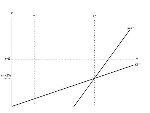
Update December 19, 2014: Although the main point of my column is to emphasize the importance of putting negative paper currency interest rates in the monetary policy toolkit now rather than a decade or two from now (with particular urgency for the European Central Bank and the Bank of Japan), I know that for many readers, the reprise of the Spring 2013 media furor about Carmen Reinhart and Ken Rogoff’s work is equally salient. Personally, I believe eliminating the zero lower bound is much more important as whether debt lowers economic growth even when it doesn’t cause a debt crisis, but the issue of debt and growth does need to be addressed as well. 

I had a chance to read Ken Rogoff’s and October 2013 FAQ http://scholar.harvard.edu/rogoff/publications/faq-herndon-ash-and-pollins-critique. Substantively, I think this is a good response to the Thomas Herndon, Michael Ash and Robert Pollin paper (linked there) that started the media furor in Spring 2013. But my own substantive concerns are not those. They are the concerns that Yichuan Wang and I detail in our two Quartz columns and two other posts on Reinhart and Rogoff’s work:

In my view, these posts by Yichuan Wang and me are a good example of how, in Clay Christensen’s terms, the disruptive innovation of the economics blogosphere is beginning to move upscale and challenge traditional economics outlets such as working papers and journal articles.

I hope that, taken as a whole, what I write on my blog puts things in the context of the literature, and—through links—gives the kinds of references that are rightly considered important for academic work. In any case, for me the major source of the not inconsiderable number of references I have had in my academically published work come from other people telling me about work related to my own. The same thing happens online. I deeply appreciate the many links people send me in tweets and in more private communications. 

Although it is natural for an individual blog post to be be much less complete than a working paper or journal article, I hope to achieve a reasonable balance between breadth and depth in this blog as a whole. And of course, the relative difficulty of putting mathematical equations in Tumblr means I will choose the working paper format once the number of equations needed to make a point exceeds a certain threshold. 

To repeat, although Thomas Herndon, Michael Ash and Robert Pollin’s paper definitely piqued my interest and Yichuan’s interest and so led to our analysis of Carmen Reinhart and Ken Rogoff’s postwar data, I am critical of the substance of Carmen and Ken’s work based on my work with Yichuan, not based on the work of Thomas Herndon, Michael Ash and Robert Pollin.

In relation to our own critique of Carmen and Ken’s work, let me make three substantive points:

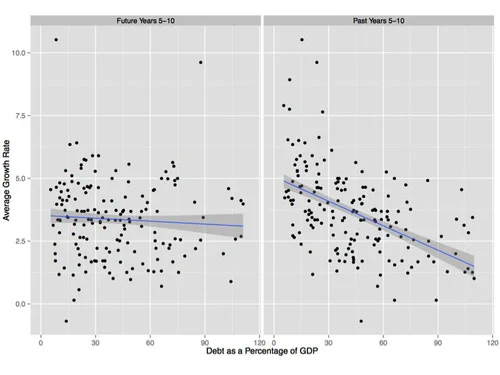
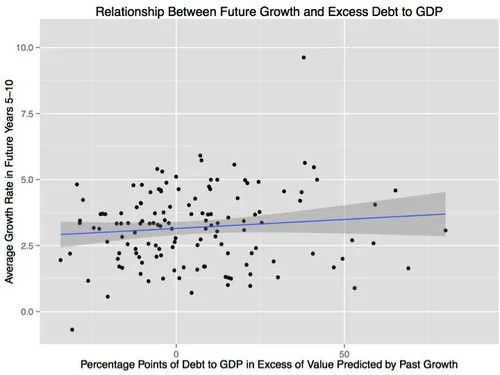
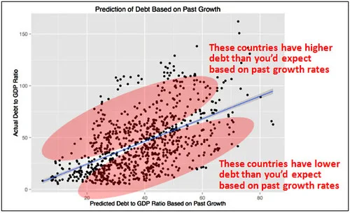
  1. Nonlinearity. In our last piece on Reinhart and Rogoff’s work, http://blog.supplysideliberal.com/post/55484991854/quartz-25-examining-the-entrails-is-there-any
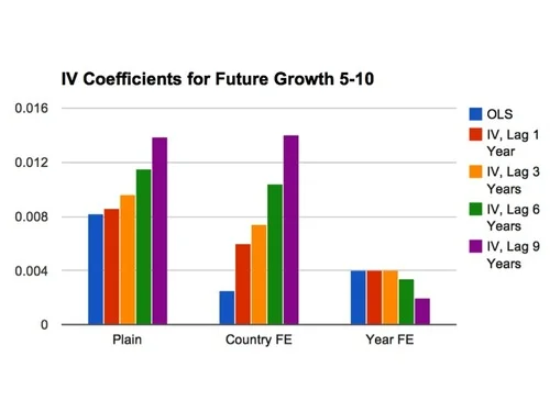
  2. Yichuan and I look nonlinearly at how different levels of debt are related to growth beyond what one would expect from looking at past growth alone. It would be nice to have more evidence total, but on its face, the hint has a higher growth rate after controlling for past growth at a 90% debt to GDP ratio than at a 50% debt to GDP ratio. And we do suggest that what little evidence there is in the data suggests that, say, 130% debt to GDP ratio is associated with lower growth beyond what would be predicted by past growth than a 90% debt to GDP ratio, though a 130% debt to GDP ratio and a 50% debt to GDP ratio give about the same level of growth beyond what would be predicted by past growth alone. On theoretical grounds, it seems plausible to me, though far from an open-and-shut case that high enough debt levels would cause problems for economics growth. That thinking has led me to argue persistently that monetary stimulus is better than fiscal stimulus because it does not raise national debt. See for example my post “Monetary vs. Fiscal Policy: Expansionary Monetary Policy Does Not Raise the Budget Deficit.”But exactly how high that is matters a lot when people can’t be convinced of the virtues of negative interest rates so that fiscal stimulus remains an issue. I consider the nonlinear smoother result that (given what power there is in the postwar data set) the line is the same at a 130% debt to GDP ratio as at a 50% debt to GDP ratio, even after correcting for “illusory growth” on the part of Ireland and Greece as painting a considerably different picture than someone would get from reading Carmen Reinhart and Ken Rogoff’s, or Carmen Reinhart, Vincent Reinhart and Ken Rogoff’s work.
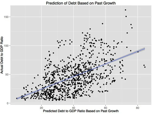
  3. Is controlling for past GDP growth appropriate? In my view, yes. I consider the past income growth controls important because countries that are generally messed up are likely to have both high debt and low growth. That doesn’t mean the high debt causes low growth. Most of the discussion has focused on reverse causality, but I consider the positive correlation across many dimensions of bad policy to be another big issue. I worry that the past income controls would make it hard to detect whether or not debt overhangs are followed by long-lasting low-growth periods, as Carmen, Vincent and Ken argue. But without some other way to control for the many, many other possible bad policies besides debt (which goes beyond the kind of growth accounting regressions that Ken’s FAQ document points to as strong evidence in favor of the view that debt might slow growth) this seems to me to point toward genuine empirical agnosticism about whether debt lowers growth as the right conclusion. (Theoretical arguments are a different matter.)
  4. Does the prewar data strongly bolster the case the debt slows growth?  Here, it depends on what the question means. The prewar data were not as readily available as the postwar data, so Yichuan and I did not analyze them. And so I don’t know what they say, once subjected to the kind of empirical exercises I would like to subject them to. I would love to see an analysis like the one the Yichuan and I did on the postwar data applied to the prewar data. That said, the prewar data may answer the question of whether a given debt level lowered growth under the gold standard, or with prewar institutions that were weaker than current institutions. So I have my doubts about how much guidance it can give to policy now. Monetary policy in particular, had advanced dramatically since the pre-World War II era, even before the ongoing revolution against the paper currency standard. 

Did Carmen and Ken overstate their case? 

While I feel confident that Yichuan’s and my substantive critique has not been adequately addressed, I am much less confident about claims I made in “Righting Rogoff on Japan’s monetary policy” about how policy-makers interpreted Carmen and Ken’s work (and how they could have been expected to have interpreted it, given what was written).

Ken’s FAQ document points to the 2010 Voxeu article “Debt and Growth Revisited” as something that could have provided more balance to policy makers in interpreting Carmen (and Vincent) and Ken’s work. Because policymakers might be more likely to read a Voxeu article than an academic paper, this Voxeu piece is an important touchstone for whether Carmen and Ken overstated the strength of the empirical evidence in favor of the idea that high public debt slows down growth in the range that was relevant to policy in the last few years.

The issue I have with the Voxeu article “Debt and Growth Revisited” is that it never mentions the fact that the normal standard of establishing causality in economics is to find a good instrument, or some other source of exogeneity or quasi-exogeneity. In other words, the inherent difficulty of establishing causality in this kind of data is never mentioned. Here is how strongly Carmen and Ken suggest in their Voxeu article “Debt and Growth Revisited” that there is causal evidence despite the highly endogenous nature of the data:

Debt-to-growth: A unilateral causal pattern from growth to debt, however, does not accord with the evidence. Public debt surges are associated with a higher incidence of debt crises.9 This temporal pattern is analysed in Reinhart and Rogoff (2010b) and in the accompanying country-by-country analyses cited therein. In the current context, even a cursory reading of the recent turmoil in Greece and other European countries can be importantly traced to the adverse impacts of high levels of government debt (or potentially guaranteed debt) on county risk and economic outcomes. At a very basic level, a high public debt burden implies higher future taxes (inflation is also a tax) or lower future government spending, if the government is expected to repay its debts.

There is scant evidence to suggest that high debt has little impact on growth. Kumar and Woo (2010) highlight in their cross-country findings that debt levels have negative consequences for subsequent growth, even after controlling for other standard determinants in growth equations. For emerging markets, an older literature on the debt overhang of the 1980s frequently addresses this theme. …

… We have presented evidence – in a multi-country sample spanning about two centuries – suggesting that high levels of debt dampen growth.

I appreciate the note of uncertainty in the sentence  

Perhaps soaring US debt levels will not prove to be a drag on growth in the decades to come.  

But I feel that for the typical policy maker reading the Voxeu article, this note of uncertainty is largely cancelled out by the next sentence: 

However, if history is any guide, that is a risky proposition and over-reliance on US exceptionalism may only prove to be one more example of the “This Time is Different” syndrome.

The phrase “if history is any guide” phrase in particular suggests that the historical evidence gives some clear guidance, and the sentence as a whole points to an interpretation of “Perhaps soaring US debt levels will not prove a drag on growth in the decades to come” as simply making a bow toward random variation around a regression line rather than expressing any uncertainty about what the causal regression line for the effect of debt on growth says before other random factors are added in.

In any case, saying “Perhaps soaring US debt levels will not prove to be a drag on growth in the decades to come” is not the same as if Carmen and Ken had said

Of course further research could overturn the suggestion we find in the evidence that high debt lowers growth, and there are always many difficulties with interpreting historical evidence of this kind.

Of course, there is always the possibility that Carmen and Ken said almost exactly that, in a forum that most policy makers would have noticed, but one that Idid not notice. (My own reading is ridiculously far from comprehensive.) If so, I would love to get a link to it. Ideally, I would like to see the main text of Ken’s FAQ document collect in its main text all the details (including of course venue or outlet and date) about all the strongest caveats and cautions against overreading that Carmen, Vincent and Ken wrote about their work. 

One extremely important note that the FAQ document does have is this quotation from Reinhart, Reinhart, and Rogoff (2012), “Public Debt Overhangs: Advanced-Economy Episodes since 1800.” (Journal of Economic Perspectives, 26(3)): 

This paper should not be interpreted as a manifesto for rapid public debt deleveraging exclusively via fiscal austerity in an environment of high unemployment. Our review of historical experience also highlights that, apart from outcomes of full or selective default on public debt, there are other strategies to address public debt overhang, including debt restructuring and a plethora of debt conversions (voluntary and otherwise). The pathway to containing and reducing public debt will require a change that is sustained over the middle and the long term. However, the evidence, as we read it, casts doubt on the view that soaring government debt does not matter when markets (and official players, notably central banks) seem willing to absorb it at low interest rates – as is the case for now.”

This suggests to me that Paul Krugman went overboard in his criticism of Carmen and Ken—at least before he backed off somewhat. I am not up on all the details, but it is my understanding that some of Paul Krugman’s stronger criticisms against Carmen and Ken in terms of providing intellectual backing for austerity might have been better leveled against other influential economists, such as Alberto Alesina. But I would need a lot of help to know whether such criticisms were even appropriate for other influential economists such as Alberto. For the record, the current Wikipedia article on Alberto Alesina says:

In October 2009 Alesina and Silvia Ardagna published Large Changes in Fiscal Policy: Taxes Versus Spending,[3] a much-cited academic paper aimed at showing that fiscal austerity measures did not hurt economies, and actually helped their recovery. In 2010 the paper Growth in a Time of Debt by Carmen Reinhart and Kenneth Rogoff) was published and widely accepted, setting the stage for the wave of fiscal austerity that swept Europe during the Great Recession. In April 2013 some analysts at the IMF and the Roosevelt Institute found the Reinhart-Rogoff paper flawed. On June 6, 2013 U.S. economist and 2008 Nobel laureatePaul Krugman published How the Case for Austerity Has Crumbled[4] in The New York Review of Books, noting how influential these articles have been with policymakers, describing the paper by the ‘Bocconi Boys’ Alesina and Ardagna (from the name of their Italian alma mater) as “a full frontal assault on the Keynesian proposition that cutting spending in a weak economy produces further weakness”, arguing the reverse.

Thus, Wikipedia conflates Carmen and Ken’s views with those of Alberto Alesina and Silvia Ardagna.

But just as Carmen and Ken’s views should not be conflated with Alberto and Silvia’s views, neither should my views be conflated with Paul Krugman’s. Soon after Thomas Herndon, Michael Ash and Robert Pollin’s paper came out, I wrote in Quartz:

Unlike what many politicians would do in similar circumstances, Reinhart and Rogoff have been forthright in admitting their errors. (See Chris Cook’s Financial Times post, “Reinhart and Rogoff Recrunch the Numbers.”) They also used their response to put forward their best argument that correcting the errors does not change their bottom line. Given the number of bloggers arguing the opposite case—that Reinhart and Rogoff’s bottom line has been destroyed—it is actually helpful for them to make their case in what has become an adversarial situation, despite their self-justifying motivation for doing so. And though I see a self-justifying motivation, I find it credible that Reinhart and Rogoff’s original error did not arise from political motivations, since as they note in their response, of their two major claims—(1) debt hurts growth and (2) economic slumps typically last a long time after a financial crisis—the claim that debt hurts growth is congenial to Republicans, while the claim that it is normal for slumps to last a long time after a financial crisis is congenial to Democrats.

The results from the fairly straightforward data analysis that Yichuan and I did made me somewhat less sympathetic to Carmen and Ken. Nevertheless, I think they spoke and wrote in good faith. Errors of omission are a different issue, and there we all stand condemned, in a hundred different directions for each of us. 

It is from the perspective that we all stand condemned for errors of omission of one type or another, that I hope my words in “Righting Rogoff on Japan’s monetary policy” are taken. I also urge you to distinguish carefully between simply reportingone side of the Spring 2013 debate about Reinhart and Rogoff’s work, and things I say on my own behalf: principally that Ken does not challenge policy-maker conventional wisdom as much as I would like to see. 

Carmen and Ken literally did not have time enough to defend themselves adequately back in Spring 2013. Now that the dust has cleared, I would be glad to see them do more to tell their side of the story. 

This update is my effort to make up for some of my own errors of omission when I wrote “Righting Rogoff on Japan’s monetary policy.” In particular, I thought wrestling with Ken’s FAQ document was the least I could do to give a little more voice to Carmen and Ken’s side of the story. (To the extent that you were persuaded by Thomas Herndon, Michael Ash and Robert Pollin’s paper, or were persuaded by unjustified accusations of bad faith on Carmen and Ken’s part, you should take a close look at that FAQ document.)

Gary Conkling on My Federal Lines of Credit Proposal

I recently stumbled across the Under the Dome, CFM Federal Lobbying blog post “Put Economic Growth on the Card, Please” by Gary Conkling, inspired by William Greider’s interview with me about my Federal Lines of Credit proposal. For my original post on Federal Lines of Credit, see “Getting the Biggest Bang for the Buck in Fiscal Policy.” That was my second post after I started this blog, right after “What is a Supply-Side Liberal?” 

On the Great Recession

I am honored to have David Andolfatto discuss my proposal for eliminating the zero lower bound in his post “Are negative interest rates really the solution?” David asks what model I have in mind when I write, for example, in “America’s Big Monetary Policy Mistake: How Negative Interest Rates Could Have Stopped the Great Recession in Its Tracks," 

Even without the ZLB [the zero lower bound on nominal interest rates], there would have been some hit from the financial crisis that ensued with the bankruptcy of Lehman Brothers on Sept. 15, 2008, but negative interest rates in the neighborhood of 4% below zero would have brought robust recovery by the end of 2009.

This post gives that model. 

One thing I will not try to do in this post is to talk about how we have actually been crawling out of the hole left by the great recession using the low-power, but not powerless tool of quantitative easing. Among instruments of monetary policy, this post considers only the current short-run safe interest rate. (I discuss some of the downsides of quantitative easing relative to negative interest rates in my ”Breaking Through the Zero Lower Bound" Powerpoint file.)

Related Work 

It is a model that I have taught in my advanced undergraduate course “Business Cycles” since the mid-90’s (see scans of student notes for two different years 1, 2), building on my academic papers

(My “Business Cycles” course is Economics 418 at the University of Michigan. Masao Ogaki has also arranged for me to teach it at Keio University in Tokyo, in August 2014.)

I am currently working on a formal treatment of the kind of issues I will address here with Bob Barsky and Rudi Bachmann. Blogging has brought home to me the policy importance of pushing that paper through to completion. We do not have a full draft yet, but if you want to see the kind of model it is, here is a mathematical appendix I put together early on in our process of writing that paper

But to understand what I am going to say, you don’t need to read the academic papers I flag above. The only indispensable prerequisite for understanding what I am going to say beyond a general background in economics is to read my post “The Medium-Run Natural Interest Rate and the Short-Run Natural Interest Rate,” where I discuss why I reject the IS-LM model on theoretical grounds, using instead the soundly micro-founded KE-MP model.

The Argument for Sticky Prices, Sticky Wages or Sticky Information or Sticky Information Processing Relevant to Prices and Wages

I am claiming that the KE-MP model is soundly “micro-founded,” but “micro-founded” is of course always a matter of degree. The Arrow-Debreu model is not fully micro-founded because it does not explain how the contracts at its heart are enforced! In the case of the KE-MP model, the place where the micro-foundations do not go as deep as one might wish is in explaining why prices are determined in the way they are. I consider the evidence of substantial monetary nonneutrality (from Friedman and Schwartz, from Romer and Romer, from vector auto-regressions, from the experience of central bankers even after allowing for some of the likely psychological biases, etc.) very persuasive. Despite many attempts, models without sticky prices, sticky wages or some kind of sticky information or sticky information processing relevant for prices and wages have not been very successful at explaining substantial monetary nonneutrality. (In saying this, I am leaving aside models that, in their totally real versions, have multiple equilibria; it is of course easy to have nominal things help select among multiple real equilibria.) Thus, regardless of the qualms one might have about why prices might be sticky (or wages, or information relevant to prices and wages), it is appropriate to assume something that is the moral equivalent of sticky prices in the broad sense.

Many people do not realize that there is another very powerful strand of evidence for something like sticky prices: the observed response of the economy to technology shocks. In “Are Technology Improvements Contractionary?”Susanto Basu, John Fernald and I make a careful, extensive, and I believe persuasive, argument that the observed response of the economy to technology shocks is very hard to square empirically with models that lack something like sticky prices, sticky wages or sticky information or sticky information processing relevant to prices and wages. I have been disappointed in the years since it was published that this aspect of our paper–this argument for sticky prices or the like–has had as little influence as it has. (Of the many citations the paper has, the bulk appear to be from economists who are simply eager to use our measure of technology shocks.)   

As for the empirical evidence behind "Are Technology Improvements Contractionary?“, it is nice to know that our evidence based on purifying Solow Residuals of variable capital and labor utilization and increasing returns to scale to identify technology shocks is backed up by the very different methodology of structural vector autoregressions of aggregate hours and output, beginning especially with Jordi Gali’s paper ”Technology, Employment, and the Business Cycle: Do Technology Shocks Explain Aggregate Fluctuations?“ (which was actually contemporaneous with our work in ”Are Technology Improvements Contractionary?“ in its inception, but was completed much more quickly than our paper), and ably defended by John Fernald in his paper Trend Breaks, Long-Run Restrictions, and Contractionary Technology Improvements.

One of the important contributions of ”Are Technology Improvements Contractionary?“ is to focus on the evidence that technology improvements are contractionary for business investment as well as for labor hours. That evidence for a contractionary effect on business investment of immediate permanent technology shocks, is actually much more decisive as evidence for something like sticky prices than the evidence of a contractionary effect on hours. (Note that if technology improvements are anticipated in advance, in a real business cycle model they should make both investment and hours increase at the moment when the technology actually improves. But both investment and hours decline when the technology is observed to improve.)

I should mention in passing that the response of the economy to technology shocks only provides evidence for sticky prices because the monetary policy response to technology shocks is suboptimal. An optimal monetary policy response to technology shocks should strive to make the economy behave like the real business cycle model corresponding to perfectly flexible prices. (In my column "Show Me the Money” I discuss the importance of monetary policy responses to tax policy changes as well as technology shocks.)

Sluggish Inflation

In the graphs I present below, I will treat inflation as being relatively sticky and unchanging. I was clued into the importance of sluggishly changing inflation by Michael Kiley’s job talk at the University of Michigan in 1995 and presented my own (never published) model to generate that kind of behavior at a seminar at Harvard in May, 2000. But given the premium on actually publishing things in academic journals, I gave this account of those ideas in my post “Trillions and Trillions: Getting Used to Balance Sheet Monetary Policy”:

I take the idea that inflation adjusts gradually from my main graduate school advisor Greg Mankiw, one of the most eminent New Keynesians: both from his textbook where he gives his view of the facts and from his theoretical 2002 paper with Ricardo Reis trying to explain those facts: “Sticky Information Versus Sticky Prices: A Proposal to Replace the New Keynesian Phillips Curve.”Michael Kiley anticipated Mankiw and Reis in his 1995 job market paper. He used the nice phrase “sluggish inflation” to describe what he was explaining with his model. 

The thing I emphasize to my graduate students is that if inflation is sticky, as distinct from the price level being sticky, that some kind of imperfect information processing must be involved. Why? Let’s think of a continuous-time model–or it is good enough to think of a model with 365 periods per year–for clarity. Inflation yesterday was generated by the firms that changed their prices yesterday. But with staggered price setting, the firms that were changing their price yesterday are different firms than the one that are changing their prices today. So, other than having a similar information environment, there is nothing connecting inflation yesterday to inflation today. If firms are optimally using all available information, and something big happens between yesterday and today, then inflation should jump, since the optimal price to change to today should generally be different than the optimal price to change to yesterday. (I am assuming that the old price firms are changing from is changing gradually at that juncture.) To make inflation not jump when something important happens requires firms today somehow not fully using that new information. That is, there has to be some form of imperfect information processing. Mankiw and Reis model the imperfect information processing as firms being asleep relative to new information and making up price changes based on old information much of the time, then periodically updating the information set they are using in full

The key evidence for sluggish inflation is how costly it seems to be to reduce inflation. Paul Krugman gives a nice (though as usual, combatively framed) description of the relevant historical episode in his very interesting post “Fighting the Last Macro War?”:

So, what were the macro wars of the last few decades? First there was stagflation — and that did indeed knock Keynesians back for a while, even as it gave freshwater macro some credibility. As I’ve already indicated, the freshwater guys then stopped there. And I mean really, really stopped there: in many ways they seem to be forever living in 1979.

In particular, they never reacted at all to the second macro war, the disinflation of the 1980s. The point there was that disinflation was very costly, with protracted high unemployment — which shouldn’t have happened if freshwater macro were at all right. This reality, as much as clever new models, drove the Keynesian revival …

What Paul doesn’t say there, but I think would agree with, is that costly disinflation is not only evidence for monetary nonneutrality, but also evidence against something as simple as the usual Calvo model of price setting, which has sticky prices, but jumping inflation. Indeed, Larry Ball among others pointed out that the Calvo model implies that disinflation brought on by a gradual reduction in the growth rate of the money supply should cause a boom if price setting were as in the usual Calvo model of price setting.

In any case, though the usual Calvo model might be OK for some pedagogical purposes, it is seriously flawed as a representation of reality in any context in which it might matter whether inflation is sluggish or not. For a recent, brief discussion of evidence for sluggish inflation in the context of the Great Recession, see Bob Hall’s strong words in “The Routes into and out of the Zero Lower Bound”:

The historical pattern is that a rise in unemployment generates a transitory decline in inflation, but the rise wears off quite quickly, and an extended period of high unemployment|as in the U.S. since 2007 has no effect on inflation.

(Note: I am not persuaded by Bob Hall’s story for why inflation has not fallen faster during the Great Recession.)

The KE-MP Model

I build the KE-MP model in “The Medium-Run Natural Interest Rate and the Short-Run Natural Interest Rate.” So far, this is the version without a zero lower bound.

The MP curve is simply the monetary policy rule, which says that at its regular meetings (every six weeks or so for the Fed) the monetary policy committee will raise the target interest rate if output is higher than at the last meeting and lower the target interest rate the Fed will raise the target interest rate if output is lower than at the last meeting.

The KE curve shows what happens as a result of equilibrium in the capital rental market. The key point is that firms will be willing to pay more to rent capital when the economy is in a boom than when the economy is in recession. Therefore, the rental rate for capital is an upward-sloping function of output. (As I discuss in The Quantitative Analytics of the Basic Neomonetarist Model, even adding a Q-theory-type investment-smoothing motive modifies this story less and less the longer-lasting a recession is. All the ins and outs of that kind of modification are one of the key issues addressed by the paper I am working on with Bob Barsky and Rudi Bachmann.)   

To begin with, think of short-run equilibrium as requiring that the short-term interest rate equal the rental rate net of depreciation. The reason is one that goes back to Dale Jorgenson: if the net rental rate is less than the real interest rate, then a firm would be better off waiting until later to invest. So it won’t invest now. If the net rental rate is higher than the real interest rate, then a firm should be eager to invest now (as long as a generic investment project meets the longer-run positive present-discounted value test–something that is guaranteed unless interest rates are expected to be above the net rental rate in the future). 

To give my view of the Great Recession, in addition to imposing the zero lower bound on the MP curve, I need to add one important wrinkle to the KE curve–a risk premium between the net rental rate and the safe interest rate. Because building a building, buying equipment or writing software or uncertain value is risky, the net rental rate actually needs to be higher than the safe short-term interest rate for a firm to invest now instead of later. Given that, I want the KE curve to represent not the net rental rate, but the risk-adjusted net rental rate–that is, the safe interest rate that is just low enough that, given the risk premium, would make firms indifferent between investing now and investing later. In many discussions with Tomas Hirst (see for example “Doubting Tomas: Electronic Money in an Open Economy with Wounded Banks”), he writes as if the relevant risk premium is infinite. In my model, it isn’t. And I don’t think the risk premium is infinite in the world either. There is some real interest rate low enough that firms will not want to delay investment until later. Nevertheless, the risk premium tends to (a) be lower in good times than in bad times, lending a higher slope to the risk-adjusted KE curve, and (b) to change for reasons other than the current level of output, causing shifts in the risk-adjusted KE curve.

The Risk-Adjusted KE Curve

To see why the relationship of the risk premium to the output gap makes the risk-adjusted KE curve more strongly upward-sloping, note that

  • at low levels of output (on the left in the graph just above), the risk-premium pushes the risk-adjusted KE curve a long way below the before-risk-adjustment KE curve

  • at high levels of output (on the right in the graph just above), the risk-premium pushes the risk-adjusted KE curve only a modest distance below the before-risk-adjustment KE curve.

From here on, the curve labeled “KE” will always be the risk-adjusted KE curve: the locus of safe short term rates that makes a typical firm indifferent between investing now and investing later on a generic investment project.   

Imposing the Zero Lower Bound on the MP Curve and Accounting for Sources of Aggregate Demand Other than Generic Investment Projects

I have written a lot about the zero lower bound and how to eliminate it. See my reader’s guide “How and Why to Eliminate the Zero Lower Bound" Graphically, since the real interest rate is the nominal interest rate minus expected inflation, if inflation is steady at 2% per year (the long-run inflation target for the Fed, the European Central Bank and the Bank of England, and currently the fond wish of the Bank of Japan), then the zero lower bound on the nominal interest imposes a lower bound of -2% per year on the real interest rate.

In addition to the KE and MP curves that govern generic investment, there is one other key element of the graph above: the level of output when generic investment is zero: Y(read "Y underbar”). When generic investment is zero, aggregate demand is composed of consumption, government purchases, net exports, and investment from special investment opportunities. 

For simplicity I am treating the special investment opportunities as so good that they will be pursued regardless of any changes in the risk-adjusted net rental rate or the real interest rate during this episode. Government purchases are exogenous. Consumption is determined by people’s views about the post-recession future according to the permanent income hypothesis. (The elasticity of intertemporal substitution in the model is low enough that interest rate effects on consumption can be ignored if interest rate fluctuations are short-lived.) If you want to think of this as a simplified model of the world economy, then net exports are zero. Alternatively, think of other country’s central banks matching most interest rate moves for the safe short-term rate, so that there is very little change in international capital flows or the closely linked value of net exports.

What is a generic investment project in the real world? I suspect it is building a house. Note that rental rates for housing, like rental rates for factories and machines, are likely to be higher in good times than in bad times. So there would still be an upward-sloping KE curve if house construction is the main component of “generic investment.” For this to work, it turns out to be crucial that house prices are sticky, even from at the moment construction commences on a house–as Bob Barsky, Chris House and I argue in our paper “Sticky Price Models and Durable Goods.” Thinking about it from the standpoint of theory, it is quite mysterious to me why house prices would be sticky, yet it seems consistent with the data to say that they are. If the typical generic investment project is building a house, then a key transmission mechanism for a typical recessions would be a partial or total shutdown of house construction.  

The 3 Equilibria in Normal Times

I am not in general a fan of multiple equilibrium models. Here, except for the zero lower bound, there would be only a single stable equilibrium. But the zero lower bound often creates two additional equilibrium. The rightmost intersection between KE and MP above is what I will call “the normal equilibrium” or “the good equilibrium.” (In the graph I have drawn the good equilibrium at the natural level of output Yn, which is where it will be in medium-run equilibrium.) The good equilibrium is the equilibrium that would remain in the absence of the zero lower bound (unless monetary policy were intentionally so tight as to push output down to Y). The good equilibrium is stable because

  • if output gets a little above that level, the central bank will raise the real interest rate above the risk-adjusted net rental rate, causing firms to start delaying investment projects that are not already underway, leading to a gradual decline in investment as investment projects already underway gradually get completed. That gradual downward adjustment of investment takes about nine months, and brings output back down to the short-run equilibrium level at the intersection of KE and MP. (See “Investment Planning Costs and the Effects of Fiscal and Monetary Policy" for the background for this gradual investment adjustment process.)

  • If output gets a little below that level, the central bank will lower the real interest rate below the risk-adjusted net rental rate, and firms will then be eager to do generic investment projects immediately–or as soon as they can be planned out. The extra aggregate demand from these additional investment projects will gradually cause output to rise back to the short-run equilibrium level at the intersection of KE and MP.

Notice that in this story, it is crucial for stability that the central bank raise its target interest more with changes in output than the rate at which the risk-adjusted net rental rate changes with changes in output. (This is a very different kind of stability issue than what is often emphasized in monetary models.) Not making the target interest rate go up strongly enough with output would lead to instability. And indeed, the intersection of the zero-lower-bound portion of the MP curve with the KE curve is an unstable equilibrium. Let me justify the label of "unstable equilibrium” that I have given to that point.

  • To the right of the intersection where the KE curve cuts the horizontal MP curve from below, the risk-adjusted net rental rate is above the real interest rate, which encourages more investment and raises leads to even higher output, leading ultimately to the normal equilibrium.

  • To the left of that intersection where the KE curve cuts the horizontal MP curve from below, the risk adjusted net rental rate is below the real interest rate, making firms want to delay all generic investment projects (according to Dale Jorgenson’s logic), leading to a decline in investment as projects already underway are completed, and a corresponding decline in output, which would only end when generic investment has been completely shut down, bringing output down to Y.

Finally at Y, there is a stable “depression equilibrium.” At that point, the risk-adjusted net rental rate is below the real interest rate, so firms want to delay all generic investment projects. Even if something made output go up a tad, the risk-adjusted net rental rate would still be strictly below the real interest rate, so firms would still want to delay all generic investment projects. With all generic investment projects delayed, output will be stuck at Y, which is the level of output that can be supported by aggregate demand from consumption, government purchases, net exports and special investment projects.

An Increase in the Risk Premium Leads to a Collapse of Generic Investment

In my model, there is no confidence fairy. Equilibrium selection is simple: once in one of the two stable equilibria, the economy stays in that equilibrium (with what ever adjustments occur to that equilibrium), unless the time comes when that equilibrium ceases to exist. The trouble is that, for a while at the end of 2008 and early 2009, the good equilibrium didcease to exist. For reasons that we understand at the same level that non-economists do, but do not understand at a deep theoretical level, the risk premium increased, and the KE curve therefore shifted down. Indeed, my view is that it shifted down enough that the the panic KE curve, labeled KE’, was everywhere below the MP curve, given the constraint imposed by the zero lower bound. With risk-adjusted net rental rate for generic investment projects everywhere below the real interest rate, generic investment began shutting down, and the economy headed toward the depression equilibrium.    

The Effects of Some Monetary Easing and Some Reduction in the Risk Premium, Subject to the Zero Lower Bound

Just above, I have drawn KE after some success of efforts to reduce the risk premium (labeling it KE’’) and MP after some monetary easing (labeling it MP’), but still subject to the zero lower bound. If all of this could have been done quickly enough, it might have been possible to get the risk-adjusted net rental rate above the real interest rate while the level of output was still above the unstable equilibrium at the intersection of the zero lower bound with the somewhat restored KE curve. But by the time these steps were completed, output was already below the level at the unstable equilibrium. Thus, the risk-adjusted net rental rate was already below the real interest rate, and the zero lower bound prevented the real interest rate falling enough to change that inequality. So the economy continued heading toward the depression equilibrium.

Eliminating the Zero Lower Bound and Going to Negative Interest Rates Leads to Recovery by the End of 2009 (What Could Have Been)

If there had been no zero lower bound, a straightforward shift downward in the MP curve to compensate for the increase in the risk premium could have kept the short-run equilibrium at the natural level of output. Here I have drawn a KE’’ curve a little higher than the KE’ curve was in order to represent some success of efforts to bring the risk premium back down, but that is not essential. However much the KE curve goes down, it is possible to shift the MP curve down just as much.

Of course, if the risk premium were going to stay high for years and years, that would have some effect on the natural level of output, but other than the delay condition highlighted in the KE-MP graph, it is only the time integral of the risk premium that matters. So a year or two of an elevated risk premium probably would not have a big effect on the natural level of output. And along with the bailouts that actually took place, and reasonable macroprudential efforts to avoid a repeat of the financial crisis, the economic recovery from effective monetary policy–unhindered by the zero lower bound–would probably have kept the effects on the risk premium quite reasonable in duration.

Let me make a few more points here. First, the reason I said the recession would be over by the end of 2009 is that it takes about 9 months for investment to adjust to changes in monetary policy. Second, there is no need to posit any technology shock to explain the Great Recession. Risk premia shocks indeed real shocks, but they differ from technology shocks in mattering for the natural level of output (the medium-run equilibrium) only in proportion to how long they are going to last. By contrast, as is well known from the Real Business Cycle literature, even a short-lived technology shock, if there were such a thing, would have a very powerful effect on the medium-run equilibrium. (In a real business cycle model, among things easy to draw in a phase diagram, a risk premium shock is more like a temporary shock to the utility discount rate.) Third, it is good to check in the graph just above that there is only one stable equilibrium; with the appropriate shift in the MP curve shown, that equilibrium is at the (mostly unchanged) natural level of output. Thus, the recession has been ended with more or less full recovery.  Finally, if the central bank doesn’t go to negative interest rates until later on, the capital stock is likely to have declined somewhat, reducing the natural level of output.

Bonus: Fiscal Policy in the KE-MP Model

I am done with my main message. And I consider fiscal policy markedly inferior as a way to deal with the kind of thing we faced in the last few years. But it is of some interest to see what the model here has to say about changes in government purchases. The first thing to say is that at the good equilibrium, increases in government purchases crowd out generic investment 1 for 1 in the short-run equilibrium. Because investment plans take time to adjust, speedy changes in government purchases could have an effect on the ultra-short-run equilibrium for about 9 months (as discussed in “Investment Planning Costs and the Effects of Fiscal and Monetary Policy”), but changes in government purchases that took just as long to plan would have no effect on output. (It is possible to get some longer-lasting effects of government purchases on output, but it requires putting more barriers in the way of adjustments in generic investment than the KE-MP model has.)

The Effects of an Increase in Government Purchases at the Zero Lower Bound

Once the economy is in the depression equilibrium, an increase in government purchases cannot crowd out generic investment because generic investment is already zero.  Thus, an increase in government purchases raises Y to Y’. For modest increases in government purchases (say, like the actual stimulus package), though this improves the depression equilibrium, it does not get the economy out of the depression equilibrium. But given some success at reducing the risk premium and loosening of monetary policy where possible above the zero lower bound, if the increase in government purchases were large enough (say three times as big as the actual stimulus package), it might push output to Y’’, as shown below, a higher level of output than the unstable equilibrium, bringing the risk-adjusted net rental rate above the -2% per year real rate at the zero lower bound, and reignite generic investment. (See below.) Note that there is critical level of government purchases that does this, and a discontinuity in the effects of government purchases at that level.     

The graph below shows a situation where efforts to bring the risk premium back down have been less successful. Here the triple-sized increase in government purchases is not enough. 

But a still bigger increase in government purchases combined with a zero nominal rate up to an even higher level of output might do the trick, as shown below.  

“Stagnation”

Of course, there is the logical possibility that the risk-adjusted net rental rate might be below -2% per year even at the natural level of output. In this situation, the zero lower bound makes it impossible to reignite generic investment (until longer-run forces intervene, such as the gradually wearing away of the generic capital stock).

How Eliminating the Zero Lower Bound Deals with Stagnation

Even the stagnation situation is compatible with getting back to the natural level of output if the zero lower bound has been eliminated. The real interest rate would be below -2% at the natural level of output, reflecting some combination of bad supply-side factors, but monetary policy would be handling those supply-side factors as gracefully as possible.

Enkhjargal Lkhagvajav: John Taylor is Wrong—Inequality *Is* Holding Back the Recovery

Enkhjargal Lkhagvajav, who goes by “Enjar"

Enkhjargal Lkhagvajav, who goes by “Enjar"

The students in my “Monetary and Financial Theory” course at the University of Michigan write 3 posts per week on an internal class blog. I liked Enjar’s post so much that I asked if I could publish it here as a guest post. Enjar said yes. I think you will find the analysis interesting. Here is what Enjar has to say:


Rising Inequality Explains the Weak Recovery, Not Vice Versa

In this article, I will not passionately try to convince you of the post title [in bold, just below the row of asterisks]. Instead, I will make points on how John B. Taylor’s argument on the topic fails under more scrutiny. In his article in the Wall Street Journal, titled ”The Weak Recovery Explains Rising Inequality, Not Vice Versa”, John B. Taylor makes following use of data to make his point that today’s inequality isn’t a cause of the type of recovery we are witnessing. First, he explains what the people who he is arguing against say: the slow recovery has been a result of growing inequality. He writes down their argument as follows:

“The key causal factor of the middle-out view is that a wider income distribution slows economic growth by lowering consumption demand. Saving rates rise and consumption falls if the share of income shifts toward the top, according to middle-out reasoning, because people with higher incomes tend to save more than those with lower incomes.”

And then he goes on to counteract this view by data he collected and put some make up on. He gives what his data shows:

“The data for the recovery since mid-2009 do not support this view. The 5.4% overall savings rate during this recovery is not high compared with the 8.4% average since 1960. It is relatively low compared to past recoveries, such as the 9.3% savings rate during a comparable period during the recovery in the early 1980s.”

In my curiosity, I was able to look at the data he worked on. It is data on personal saving ratio-the ratio of personal saving to disposable personal income. The following graph shows what the saving rate has been.

John Taylor is correct on that the saving rate has been averaging 5.4% since the end of the latest recession. However, when he tried to compare this rate to the 8.4% average rate since the 1960, he makes wrong comparison. Due to the general downward trend of this rate over the last decades, he shouldn’t compare this 5.4% average rate of saving during the recovery to the all time average saving rate. But if we compare the 5.4% average rate during the recovery with the average saving rate between the end of 2001 and the start of the recession, which is 3.9%, we can see that the saving rate today is higher than its pre-recession level. Therefore, we have just disproved his claim by using the same argument he tried to use. In other words, with data on how the income inequality has grown, we have further see that the saving rate also increased after the recession.

Hence, we are able to claim that the increase in inequality indeed increased the saving rate; therefore, the total consumption demand has declined, which is exactly what the people he argued against said.

One could argue that increased personal saving rate isn’t caused by the increasing inequality . It is possible that because people might be willing to save more than what it was saving before the crisis to use their saving when another crisis comes during the recovery and uncertainty. Therefore, one could say inequality isn’t playing a much role in hindering a recovery today.

However, this surge in the saving rate after any given recession has been witnessed only twice, once after 2001 and again after 2007-2009 recessions.  The prior recoveries experienced the saving rate which was actually lower than its level before the crises. If we look at the average saving rate between November 1970 and November 1973, it was 12.8% which is higher than the saving rate after the recession, between April 1975 to December 1979, which is 10.8%. The same decrease in the saving rate was seen also during the early 1980′s recovery. We can see this trend of decrease in the saving rate following any recession in the above graph except for the last two recoveries. In last two recoveries, the saving rate surged and stayed at the higher level than it was before the recessions.

In my very first blog post, I compared the income inequality during the pre-recession periods for the Great Depression and the Great Recession and argued the recovery the economy is going through now is unhealthy one. One could agree with John Taylor on that the weak recovery is causing the widening inequality and the first problem policymakers should tackle is to boost the recovery by any means. However, the increasing inequality could be the heart of the problem, and the policymakers should prioritize equality to change the speed of the recovery. But how the inequality must be tackled should be devoted to a number of blog posts itself. I believe recent discussions and steps toward solving the inequality is a way to fasten the recovery.

Monetary vs. Fiscal Policy: Expansionary Monetary Policy Does Not Raise the Budget Deficit

Monetary policy and fiscal policy are not equally good as ways to stimulate the economy. Traditional monetary policy (that is, lowering the short-term interest rate) has two key advantages over traditional fiscal policy:

  • It does not add to the national debt
  • Because many governments have–however controversially–been willing to let monetary policy be handled by an independent central bank, it is not doomed to be tangled up in politics to the same extent that discretionary fiscal policy inevitably gets tangled up in long-running political disputes about taxing and spending.

My subtitle “Expansionary Monetary Policy Does Not Raise the Budget Deficit” is a quotation from Alan Blinder’s October 25, 2010 Wall Street Journal op-ed “Our Fiscal Policy Paradox,” where Alan also points to the political difficulties of using discretionary fiscal for macroeconomic stabilization:

The practice of monetary and fiscal policy is fraught with difficulties, but the central concept is straightforward, compelling and, by the way, 75 years old: The government should push the economy forward when unemployment is high and slow it down when inflation threatens.
To do so, governments normally have two principal sets of weapons. Fiscal policy means moving some taxes or elements of public spending up or down to either propel or restrain total spending. In the United States, such decisions are made politically, by Congress and the president. Monetary policy normally (but not now) means lowering or raising short-term interest rates to either speed up growth or slow it down. That power, of course, resides in the technocratic Federal Reserve….
There are plenty of powerful weapons left in the fiscal-policy arsenal. But Congress is tied up in partisan knots that will probably get worse after the election….
But what about using monetary policy? Chairman Ben Bernanke and his Federal Reserve colleagues are not paralyzed by politics. They have not fallen victim to misleading advertising claiming that past policies have not helped. And expansionary monetary policy does not raise the budget deficit. So why the hesitation?

Monetary Policy. My view is that we need tools for macroeconomic stabilization that (a) can be applied technocratically and (b) do not add greatly to national debt when they are used to stimulate the economy. Monetary policy fills that bill, once it is unhobbled by eliminating the zero lower bound. Here is what I wrote in my column “Why Austerity Budgets Won’t Save Your Economy”:

For the US, the most important point is that using monetary policy to stimulate the economy does not add to the national debt and that even when interest rates are near zero, the full effectiveness of monetary policy can be restored if we are willing to make a legal distinction between paper currency and electronic money in bank accounts—treating electronic money as the real thing, and putting paper currency in a subordinate role….
Without the limitations on monetary policy that come from our current paper currency policy, the Fed could lower interest rates enough (even into negative territory for a few quarters if necessary) to offset the effects of even major tax increases and government spending cuts.

The Costs of National Debt. That column is also important in giving some of the best arguments I know for worrying about the national debt now that it is hard to argue that national debt slows economic growth. (On the effect of national debt on economic growth, see my two columns with Yichuan Wang “After Crunching Reinhart and Rogoff’s Data, We Found No Evidence High Debt Slows Growth” and Examining the Entrails: Is There Any Evidence for an Effect of Debt on Growth in the Reinhart and Rogoff Data? and the other work they flag.) Here is what I had to say about the costs of debt in "Why Austerity Budgets Won’t Save Your Economy“:

…lenders are showing no signs of doubting the ability of the US government to pay its debts. But there can be costs to debt even if no one ever doubts that the US government can pay it back.
To understand the other costs of debt, think of an individual going into debt. There are many appropriate reasons to take on debt, despite the burden of paying off the debt:
  • To deal with an emergency—such as unexpected medical expenses—when it was impossible to be prepared by saving in advance.
  • To invest in an education or tools needed for a better job.
  • To buy an affordable house or car that will provide benefits for many years.
There is one more logically coherent reason to take on debt—logically coherent but seldom seen in the real world:
  • To be able to say with contentment and satisfaction in one’s impoverished old age, “What fun I had when I was young!”
In theory, this could happen if when young, one had a unique opportunity for a wonderful experience—an opportunity that is very rare, worth sacrificing for later on. Another way it could happen is if one simply cared more in general about what happened in one’s youth than about what happened in one’s old age.
Tax increases and government spending cuts are painful. Running up the national debt concentrates and intensifies that pain in the future. Since our budget deficits are not giving us a uniquely wonderful experience now, to justify running up debt, that debt should be either (i) necessary to avoid great pain now, or (ii) necessary to make the future better in a big enough way to make up for the extra debt burden. The idea that running up debt is the only way to stimulate an economic recovery when interest rates are near zero is exactly what I question… If reforming the way we handle paper currency made it clear that running up the debt is not necessary to stimulate the economy, what else could justify increasing our national debt? In that case, only true investments in the future would justify more debt: things like roads, bridges, and scientific knowledge that would still be there in the future yielding benefits—benefits for which our children and we ourselves in the future will be glad to shoulder the burden of debt.

National Lines of Credit: I write about the importance of stabilization policy that can be applied technocratically, without getting tangled up in politics in the context of my other main proposal for stabilization policy: National Lines of Credit (or equivalently "Federal Lines of Credit”). The key post there is “Preventing Recession-Fighting from Becoming a Political Football.” In any case, I think National Lines of Credit would get less tangled up in politics than regular traditional fiscal policy, but it would also be possible to set them up so that they were initiated in an explicitly technocratic way. Here is the relevant passage from my working paper “Getting the Biggest Bang for the Buck in Fiscal Policy”:

The lack of legal authority for central banks to issue national lines of credit is not set in stone. Indeed, for the sake of speed in reacting to threatened recessions, it could be quite valuable to have legislation setting out many of the details of national lines of credit but then authorizing the central bank to choose the timing and (up to some limit) the magnitude of issuance. Even when the Fed funds rate or its equivalent is far from its zero lower bound at the beginning of a recession, the effects of monetary policy take place with a significant lag (partly because of the time it takes to adjust investment plans), while there is reason to think that consumption could be stimulated quickly through the issuance of national lines of credit. Reflecting the fact that national lines of credit lie between traditional monetary and traditional fiscal policy, the rest of the government would still have a role both in establishing the magnitude of this authority and perhaps in mandating the issuance of additional lines of credit over the central bank’s objection (with the overruled central bank free to use contractionary monetary policy for a countervailing effect on aggregate demand).

Though not as good as monetary stimulus, National Lines of Credit are also much better than traditional fiscal policy in yielding a high ratio of stimulus to the amount ultimately added to the national debt.

National Rainy Day Accounts. There is a related mode of stabilization policy that I consider superior to National Lines of Credit. The National Rainy Day Accounts described in this passage of my working paper “Getting the Biggest Bang for the Buck in Fiscal Policy” would not add to the national debt at all: 

It is also worth pointing out that, in principle, national lines of credit in times of low demand could be superseded in the long run (at least in part) by a modest level of forced saving in times of high demand,  with the funds from these “national rainy day accounts” released to households in time of recession (and also perhaps in the case of one of a well-defined list of documentable personal financial emergencies).

The National Rainy Day Accounts also have household finance benefits for people who have difficulty saving for emergencies without some external discipline. The main limitations of National Rainy Day Accounts as stabilization policy is (a) that they require advance preparation and (b) the resources of National Rainy Day Accounts might sometimes be exhausted before getting enough stimulus.

Quartz #25—>Examining the Entrails: Is There Any Evidence for an Effect of Debt on Growth in the Reinhart and Rogoff Data?

Link to the Column on Quartz

Here is the full text of my 25th Quartz column, that I coauthored with Yichuan Wang, “Autopsy: Economists looked even closer at Reinhart and Rogoff’s data–and the results might surprise you.” It is now brought home to supplysideliberal.com (and soon to Yichuan’s Synthenomics). It was first published on May 14, 2013. Links to all my other columns can be found here.

If you want to mirror the content of this post on another site, that is possible for a limited time if you read the legal notice at this link and include both a link to the original Quartz column and the following copyright notice:

© June 12, 2013: Miles Kimball and Yichuan Wang, as first published on Quartz. Used by permission according to a temporary nonexclusive license expiring June 30, 2014. All rights reserved.

(Yichuan has agreed to extend permission on the same terms that I do.)


In order to predict the future, the ancient Romans would often sacrifice an animal, open up its guts and look closely at its entrails. Since the discovery of an Excel spreadsheet error in Carmen Reinhart and Ken Rogoff’s analysis of debt and growth by University of Massachusetts at Amherst graduate student Thomas Herndon and his professors Michael Ash and Robert Pollin, many economists have taken a cue from the Romans with the Reinhart and Rogoff data to see if there is any hint of an effect of high levels of national debt on economic growth. The two of us gave our first take in analyzing the Reinhart and Rogoff data in our May 29, 2013 column. We wrote that “…we could not find even a shred of evidence in the Reinhart and Rogoff data for a negative effect of government debt on growth.

Our further analysis since then (here, and here), and University of Massachusetts at Amherst Professor Arindrajit Dube’s analysis since then and full release of his previous work (herehere, and here) in response to our column have only confirmed that view. (Links to other reactions to our earlier column can be found here.) Indeed, although we have found no shred of evidence for a negative effect of government debt on growth in the Reinhart and Rogoff data, the two of us have found at least a mirage of a positive effect of debt on growth, as shown in the graph above.

The point of the graph at the top is to find out if the ratio of debt has any relationship to GDP growth, after isolating the part of GDP growth that can’t be predicted by past GDP growth alone. Let us give two examples of why it might be important to adjust for past growth rates when looking at the effect of debt on growth. First, if a country is run badly in other ways, is likely to grow slowly whatever its level of debt. In order to see if debt makes things worse, it is crucial to adjust for the fact that it was growing slowly to begin with. Second, if a country is run well, it is likely to grow fast while it is in the “catch-up” phase of copying proven techniques from other countries. Then as it gets closer to the technological frontier, its growth will naturally slow down. If getting richer in this way also tends to lead through typical political dynamics to a larger welfare state with higher levels of debt, one would see high levels of debt during that later mature phase of slower growth. This is not debt causing slow growth, but economic development having two separate effects: the slowdown in growth as a country nears the technological frontier, and the development of a welfare state. Adjusting for past growth helps us adjust for how far along a country is in its growth trajectory.

In the graph, if “GDP Growth Relative to Par” is positive, it means GDP growth is higher in the next 10 years than would be predicted by past GDP growth alone. If “GDP Growth Relative to Par” is negative, it means GDP growth is lower in the next 10 years than would be predicted by past GDP growth. (Here, in accounting for the effect of past GDP growth, we use data on the most recent five past years individually, and the average growth rate over the period from 10 years in the past to five years in the past.) The thick red line shows that, overall, high debt is associated with GDP growth just a little higher than what one would guess from looking at the past record of GDP growth alone. The thick blue curve gives more detail by showing in a flexible way what levels of debt are associated with above par growth and what levels of debt are associated with below par growth. We generated it with standard scatterplot smoothing techniques. The thick blue curve shows that, in particular, GDP growth seems surprisingly high in the range from debt about 60% of GDP to debt about 120% of GDP. Higher and lower debt levels are associated with future growth that is somewhat lower than would be predicted by looking at past growth alone. Interestingly, debt at 90% of GDP, instead of being a cliff beyond which the growth performance looks much worse, looks like the top of a gently rounded hill. If one took the tiny bit of evidence here much, much more seriously than we do, it would suggest that debt below 90% of GDP is just as bad as debt above 90% of GDP, but that neither is very bad.

Where does the evidence of above par growth in the range from 60% to 120% of GDP come from? Part of the answer is Ireland. In particular, all but one of the cases when GDP growth was more than 2.5% per year above what would be expected from looking at past growth occurred in a 10-year period after Ireland had a debt to GDP ratio in the range from 60% to 120% of GDP. It is well-known that Ireland has recently gotten into trouble because of its debt, but what does the overall picture of its growth performance over the last few decades look like? Here is a graph of Ireland’s per capita GDP from the Federal Reserve Bank of St. Louis data base:

The consequences of debt have reversed some of Ireland’s previous growth, but it is still a growth success story, despite the high levels of debt it had in the 1980s and ’90s.

In addition to Ireland, a bit of the evidence for good growth performance following high levels of debt comes from Greece. As the graph below shows, Greece has had more impressive growth in the last two decades than many people realize, despite the hit it has taken recently because of its debt troubles.

We did a simple exercise to see if the bump up in the thick blue curve in the graph at the top is entirely due to Ireland’s and Greece’s growth that has been reversed recently because of their debt troubles.  To be sure that the bad consequences of Ireland’s and Greece’s debt for GDP in the last few years were accounted for when looking at the effect of debt on growth, we pretended that the recent declines in GDP had been spread out as a drag on growth over the period from 1990 to 2007 instead of happening in the last few years. Then we redid our analysis. Making this adjustment to the growth data is a simple, if ad hoc, way of trying to make sure that the consequences of Irish and Greek debt are not missed by the analysis.

Imagining slower growth earlier on to account for Ireland’s and Greece’s recent GDP declines makes the performance of Ireland and Greece in that period from 1990 to 2007 look less stellar. The key effect is on the thick blue curve estimating the effect of debt on growth. Looking closely at the graph below after adjusting Ireland’s and Greece’s growth rates, you can see that the bump up in the thick blue curve in the range where debt is between 60% and 120% of GDP has been cut down to size, but it is still there. So the bump cannot be attributed entirely to Ireland and Greece “stealing growth from the future” with their high levels of debt.

We want to stress that there is no real justification for making the adjustment for Ireland and Greece that we made except as a way of showing that the argument that Ireland and Greece had high growth in the 1990s and early 2000s, but now have had to pay the piper is not enough to turn the story about the effects of debt on growth around.

There are three broader points to make from this discussion of Ireland and Greece.

  • We still don’t recommend taking the upward bump in growth predicted by the thick blue curves in the 60% to 120% ranges for debt seriously.
  • The fact that looking at the experience of two countries in two decades can account for a good share of the bump up in the 60% to 120% ranges illustrates just how little there is to go on from the Reinhart and Rogoff data set. Our scatter plots with the thick blue curves give the impression of more than there really is, because we have dots for growth from 1970 to 1980 and 1971 to 1981 and 1972 to 1982, and so on. And there is no way to escape this kind of issue when the economic forces one is interested have both short-run and long-run effects, and change as slowly over time as levels of national debt do. There are advanced statistical methods for correcting for such issues; the corrections almost always go in the direction of saying that there is less evidence in a set of data than it might seem. Even without being experts ourselves in making those statistical corrections, we feel reasonably confident in saying that the Reinhart and Rogoff data speak very softly about any positive or negative effect of debt on growth at all: barely a whisper.
  • Third, the inclusion of Ireland and Greece and the fact that the basic story survives after pretending their GDP declines were a drag on growth earlier contradicts to some extent the claim of economics blogger and blog critic Paul Andrews in his post “None the Wiser After Reinhart, Rogoff, et al.” that Reinhart and Rogoff’s data focus on “20 or so of the most healthy economies the world has ever seen.” After adjusting for the hit their economies have taken recently, the inclusion of Ireland and Greece gives some perspective on the effects of debt on the growth of economies that havesubsequently had problems paying for their debt. There could certainly be other economies whose growth is more vulnerable to debt than Ireland and Greece, but to us these seem like exactly the kinds of cases people would have in mind when they argue that one should expect debt to have a negative effect on growth.

Understanding all of this matters because, as Mark Gongloff of Huffington Postwrites:

Reinhart and Rogoff’s 2010 paper, “Growth in a Time of Debt,” … has been used to justify austerity programs around the world. In that paper, and in many other papers, op-ed pieces and congressional testimony over the years, Reinhart and Rogoff have warned that high debt slows down growth, making it a huge problem to be dealt with immediately. The human costs of this error have been enormous.

Even though there are many effective ways to stimulate economies without adding much to their national debt, the primary remedies for sluggish economies that are actually on the table politically are those that do increase national debt, so it matters whether people think debt is damning or think debt is just debt.  It is painful enough that debt has to be paid back (with some combination of interest and principal), and high levels of debt may help cause debt crises like those we have seen for Ireland and Greece. But the bottom line from our examination of the entrails is that the omens and portents in the Reinhart and Rogoff data do not back up the argument that debt has a negative effect on economic growth.

Quartz #24—>After Crunching Reinhart and Rogoff's Data, We Found No Evidence High Debt Slows Growth

Link to the Column on Quartz

Here is the full text of my 24th Quartz column, that I coauthored with Yichuan Wang, “After crunching Reinhart and Rogoff’s data, we’ve concluded that high debt does not slow growth.” It is now brought home to supplysideliberal.com (and soon to Yichuan's Synthenomics). It was first published on May 29, 2013. Links to all my other columns can be found here. In particular, don’t miss the follow-up column “Examining the Entrails: Is There Any Evidence for an Effect of Debt on Growth in the Reinhart and Rogoff Data?

If you want to mirror the content of this post on another site, that is possible for a limited time if you read the legal notice at this link and include both a link to the original Quartz column and the following copyright notice:

© May 29, 2013: Miles Kimball and Yichuan Wang, as first published on Quartz. Used by permission according to a temporary nonexclusive license expiring June 30, 2014. All rights reserved.

(Yichuan has agreed to extend permission on the same terms that I do.)

This column had a strong response. I have included the text of my companion column, with links to many of the responses after the text of the column itself. (For the comments attached to that companion post, you will still have to go to the original posting.) Other followup posts can be found in my “Short-Run Fiscal Policy” sub-blog.  


Leaving aside monetary policy, the textbook Keynesian remedy for recession is to increase government spending or cut taxes. The obvious problem with that is that higher government spending and lower taxes tend to put the government deeper in debt. So the announcement on April 15, 2013 by University of Massachusetts at Amherst economists Thomas Herndon, Michael Ash and Robert Pollin that Carmen Reinhart and Ken Rogoff had made a mistake in their analysis claiming that debt leads to lower economic growth has been big news. Remarkably for a story so wonkish, the tale of Reinhart and Rogoff’s errors even made it onto the Colbert Report. Six weeks later, discussions of Herndon, Ash and Pollin’s challenge to Reinhart and Rogoff continue in earnest in the economics blogosphere, in the Wall Street Journal, and in the New York Times.

In defending the main conclusions of their work, while conceding some errors, Reinhart and Rogoff point out that even after the errors are corrected, there is a substantial negative correlation between debt levels and economic growth. That is a fair description of what Herndon, Ash and Pollin find, as discussed in an earlier Quartz column, “An Economist’s Mea Culpa: I relied on Reinhardt and Rogoff.” But, as mentioned there, and as Reinhart and Rogoff point out in their response to Herndon, Ash and Pollin, there is a key remaining issue of what causes what. It is well known among economists that low growth leads to extra debt because tax revenues go down and spending goes up in a recession. But does debt also cause low growth in a vicious cycle? That is the question.

We wanted to see for ourselves what Reinhart and Rogoff’s data could say about whether high national debt seems to cause low growth. In particular, we wanted to separate the effect of low growth in causing higher debt from any effect of higher debt in causing low growth. There is no way to do this perfectly. But we wanted to make the attempt. We had one key difference in our approach from many of the other analyses of Reinhart and Rogoff’s data: we decided to focus only on long-run effects. This is a way to avoid getting confused by the effects of business cycles such as the Great Recession that we are still recovering from. But one limitation of focusing on long-run effects is that it might leave out one of the more obvious problems with debt: the bond markets might at any time refuse to continue lending except at punitively high interest rates, causing debt crises like that have been faced by Greece, Ireland, and Cyprus, and to a lesser degree Spain and Italy. So far, debt crises like this have been rare for countries that have borrowed in their own currency, but are a serious danger for countries that borrow in a foreign currency or share a currency with many other countries in the euro zone.

Here is what we did to focus on long-run effects: to avoid being confused by business-cycle effects, we looked at the relationship between national debt and growth in the period of time from five to 10 years later. In their paper “Debt Overhangs, Past and Present,” Carmen Reinhart and Ken Rogoff, along with Vincent Reinhart, emphasize that most episodes of high national debt last a long time. That means that if high debt really causes low growth in a slow, corrosive way, we should be able to see high debt now associated with low growth far into the future for the simple reason that high debt now tends to be associated with high debt for quite some time into the future.

Here is the bottom line. Based on economic theory, it would be surprising indeed if high levels of national debt didn’t have at least some slow, corrosive negative effect on economic growth. And we still worry about the effects of debt. But the two of us could not find even a shred of evidence in the Reinhart and Rogoff data for a negative effect of government debt on growth.

The graphs at the top show show our first take at analyzing the Reinhardt and Rogoff data. This first take seemed to indicate a large effect of low economic growth in the past in raising debt combined with a smaller, but still very important effect of high debt in lowering later economic growth. On the right panel of the graph above, you can see the strong downward slope that indicates a strong correlation between low growth rates in the period from ten years ago to five years ago with more debt, suggesting that low growth in the past causes high debt. On the left panel of the graph above, you can see the mild downward slope that indicates a weaker correlation between debt and lower growth in the period from five years later to ten years later, suggesting that debt might have some negative effect on growth in the long run. In order to avoid overstating the amount of data available, these graphs have only one dot for each five-year period in the data set. If our further analysis had confirmed these results, we were prepared to argue that the evidence suggested a serious worry about the effects of debt on growth. But the story the graphs above seem to tell dissolves on closer examination.

Given the strong effect past low growth seemed to have on debt, we felt that we needed to take into account the effect of past economic growth rates on debt more carefully when trying to tease out the effects in the other direction, of debt on later growth. Economists often use a technique called multiple regression analysis (or “ordinary least squares”) to take into account the effect of one thing when looking at the effect of something else. Here we are doing something that is quite close both in spirit and the numbers it generates for our analysis, but allows us to use graphs to show what is going on a little better.

The effects of low economic growth in the past may not all come from business cycle effects. It is possible that there are political effects as well, in which a slowly growing pie to be divided makes it harder for different political factions to agree, resulting in deficits. Low growth in the past may also be a sign that a government is incompetent or dysfunctional in some other way that also causes high debt. So the way we took into account the effects of economic growth in the past on debt—and the effects on debt of the level of government competence that past growth may signify—was to look at what level of debt could be predicted by knowing the rates of economic growth from the past year, and in the three-year periods from 10 to 7 years ago, 7 to 4 years ago and 4 to 1 years ago. The graph below, labeled “Prediction of Debt Based on Past Growth” shows that knowing these various economic growth rates over the past 10 years helps a lot in predicting how high the ratio of national debt to GDP will be on a year by year basis. (Doing things on a year by year basis gives the best prediction, but means the graph has five times as many dots as the other scatter plots.) The “Prediction of Debt Based on Past Growth” graph shows that some countries, at some times, have debt above what one would expect based on past growth and some countries have debt below what one would expect based on past growth. If higher debt causes lower growth, then national debt beyond what could be predicted by past economic growth should be bad for future growth.

Our next graph below, labeled “Relationship Between Future Growth and Excess Debt to GDP” shows the relationship between a debt to GDP ratio beyond what would be predicted by past growth and economic growth 5 to 10 years later. Here there is no downward slope at all. In fact there is a small upward slope. This was surprising enough that we asked others we knew to see what they found when trying our basic approach. They bear no responsibility for our interpretation of the analysis here, but Owen Zidar, an economics graduate student at the University of California, Berkeley, and Daniel Weagley, graduate student in finance at the University of Michigan were generous enough to analyze the data from our angle to help alert us if they found we were dramatically off course and to suggest various ways to handle details. (In addition, Yu She, a student in the master’s of applied economics program at the University of Michigan proofread our computer code.)  We have no doubt that someone could use a slightly different data set or tweak the analysis enough to make the small upward slope into a small downward slope. But the fact that we got a small upward slope so easily (on our first try with this approach of controlling for past growth more carefully) means that there is no robust evidence in the Reinhart and Rogoff data set for a negative long-run effect of debt on future growth once the effects of past growth on debt are taken into account. (We still get an upward slope when we do things on a year-by-year basis instead of looking at non-overlapping five-year growth periods.)

Daniel Weagley raised a very interesting issue that the very slight upward slope shown for the “Relationship Between Future Growth and Excess Debt to GDP” is composed of two different kinds of evidence. Times when countries in the data set, on average, have higher debt than would be predicted tend to be associated with higher growth in the period from five to 10 years later. But at any time, countries that have debt that is unexpectedly high not only compared to their own past growth, but also compared to the unexpected debt of other countries at that time, do indeed tend to have lower growth five to 10 years later. It is only speculating, but this is what one might expect if the main mechanism for long-run effects of debt on growth is more of the short-run effect we mentioned above: the danger that the “bond market vigilantes” will start demanding high interest rates. It is hard for the bond market vigilantes to take their money out of all government bonds everywhere in the world, so having debt that looks high compared to other countries at any given time might be what matters most.

Our view is that evidence from trends in the average level of debt around the world over time are just as instructive as evidence from the cross-national evidence from debt in one country being higher than in other countries at a given time. Our last graph (just above) shows what the evidence from trends in average levels over time looks like. High debt levels in the late 1940s and the 1950s were followed five to 10 years later with relatively high growth.  Low debt levels in the 1960s and 1970s were followed five to 10 years later by relatively low growth. High debt levels in the 1980s and 1990s were followed five to 10 years later by relatively high growth. If anyone can come up with a good argument for why this evidence from trends in the average levels over time should be dismissed, then only the cross-national evidence about debt in one country compared to another would remain, which by itself makes debt look bad for growth. But we argue that there is not enough justification to say that special occurrences each year make the evidence from trends in the average levels over time worthless. (Technically, we don’t think it is appropriate to use “year fixed effects” to soak up and throw away evidence from those trends over time in the average level of debt around the world.)

We don’t want anyone to take away the message that high levels of national debt are a matter of no concern. As discussed in “Why Austerity Budgets Won’t Save Your Economy,” the big problem with debt is that the only ways to avoid paying it back or paying interest on it forever are national bankruptcy or hyper-inflation. And unless the borrowed money is spent in ways that foster economic growth in a big way, paying it back or paying interest on it forever will mean future pain in the form of higher taxes or lower spending.

There is very little evidence that spending borrowed money on conventional Keynesian stimulus—spent in the ways dictated by what has become normal politics in the US, Europe and Japan—(or the kinds of tax cuts typically proposed) can stimulate the economy enough to avoid having to raise taxes or cut spending in the future to pay the debt back. There are three main ways to use debt to increase growth enough to avoid having to raise taxes or cut spending later:

1. Spending on national investments that have a very high return, such as in scientific research, fixing roads or bridges that have been sorely neglected.

2. Using government support to catalyze private borrowing by firms and households, such as government support for student loans, and temporary investment tax credits or Federal Lines of Credit to households used as a stimulus measure.

3. Issuing debt to create a sovereign wealth fund—that is, putting the money into the corporate stock and bond markets instead of spending it, as discussed in “Why the US needs its own sovereign wealth fund.” For anyone who thinks government debt is important as a form of collateral for private firms (see “How a US Sovereign Wealth Fund Can Alleviate a Scarcity of Safe Assets”), this is the way to get those benefits of debt, while earning more interest and dividends for tax payers than the extra debt costs. And a sovereign wealth fund (like breaking through the zero lower bound with electronic money) makes the tilt of governments toward short-term financing caused by current quantitative easing policies unnecessary.

But even if debt is used in ways that do require higher taxes or lower spending in the future, it may sometimes be worth it. If a country has its own currency, and borrows using appropriate long-term debt (so it only has to refinance a small fraction of the debt each year) the danger from bond market vigilantes can be kept to a minimum. And other than the danger from bond market vigilantes, we find no persuasive evidence from Reinhart and Rogoff’s data set to worry about anything but the higher future taxes or lower future spending needed to pay for that long-term debt. We look forward to further evidence and further thinking on the effects of debt. But our bottom line from this analysis, and the thinking we have been able to articulate above, is this: Done carefully, debt is not damning. Debt is just debt.


Companion Post

The title chosen by our editor is too strong, but not so much so that I objected to it; the title of this post is more accurate.

Yichuan only recently finished his first year at the University of Michigan. Yichuan’s blog is Synthenomics. You can see Yichuan on Twitter here. Let me say already that from reading Yichuan’s blog and working with him on this column, I know enough to strongly recommend Yichuan for admission to any Ph.D. program in economics in the world. He should finish has bachelor’s degree first, though.

I genuinely went into our analysis expecting to find evidence that high debt does cause low growth, though of course, to a much smaller extent than low growth causes high debt. I was fully prepared to argue (first to Yichuan and then to the world) that even a statistically insignificant negative effect of debt on growth that was plausibly causal had to be taken seriously from a Bayesian perspective. Our analysis set out the minimal hurdles I felt had to be jumped over to convince me that there was some solid evidence that high debt causes low growth. A key jump was not completed. That shifted my views.

I hope others will try to replicate our findings. That should let me rest easier.

From a theoretical point of view, I am especially intrigued by the possibility that any effect on growth from refinancing difficulties might depend on a country’s debt to GDP ratio compared to that of other countries. What I find remarkable is that despite the likely negative effect of debt on growth from refinancing difficulties, we found no overall negative effect of debt on growth. It is as if there is some other, positive effect of debt on growth to the extent a country’s relative debt position stays the same. Besides the obvious, but uncommonly realized, possibility of very wisely deployed deficit spending, I can think of two intriguing mechanisms that could generate such an effect. First, from a supply-side point of view, lower tax rates now could make growth look higher now, perhaps at the expense of growth at some future date when taxes have to be raised to pay off the debt, with interest. Second, government debt increases the supply of liquid (and often relatively safe) assets in the economy that can serve as good collateral. Any such effect could be achieved without creating a need for higher future taxes or lower future spending by investing the money raised in corporate stocks and bonds through a sovereign wealth fund.

I have thought a little about why borrowing in a currency one can print unilaterally makes such a difference to the reactions of the bond market to debt. One might think that the danger of repudiating the implied real debt repayment promises by inflation would mean the risks to bondholders for debt in one’s own currency would be almost the same as for debt in a foreign currency or a shared currency like the euro. But it is one thing to fear actual disappointing real repayment spread over some time and another thing to have to fear that the fear of other bondholders will cause a sudden inability of a government to make the next payment at all.  

Note: Brad Delong writes:

Miles Kimball and Yichuan Wang confirm Arin Dube: Guest Post: Reinhart/Rogoff and Growth in a Time Before Debt | Next New Deal:

As I tweeted,

  1. .@delong undersells our results. I would have read Arin Dube’s results alone as saying high debt *does* slow growth.

  2. *Of course* low growth causes debt in a big way. But we need to know if high debt causes low growth, too. No ev it does!

In tweeting this, I mean,if I were convinced Arin Dube’s left graph were causal, the left graph seems to suggest that higher debt causes low growth in a very important way, though of course not in as big a way as slow growth causes higher debt. If it were causal, the left graph suggests it is the first 30% on the debt to GDP ratio that has the biggest effect on growth, not any 90% threshold. Yichuan and I are saying that the seeming effect of the first 30% on the debt to GDP ratio could be due in important measure to the effect of growth on debt, plus some serial correlation in growth rates. The nonlinearity could come from the fact that it takes quite high growth rates to keep a country from have some significant amounts of debt—as indicated by Arin Dube’s right graph, which is more likely to be primarily causal.

By the way, I should say that Yichuan and I had seen the Rortybomb piece on Arin Dube’s analysis, but we were not satisfied with it. But I want to give credit for this as a starting place for Yichuan and me in our thinking.

Brad Delong’s Reply: Thanks to Brad DeLong for posting the note above as part of his post “DeLong Smackdown Watch: Miles Kimball Says That Kimball and Wang is Much Stronger than Dube.”

Brad replies:

From my perspective, I tend to say that of course high debt causes low growth—if high debt makes people fearful, and leads to low equity valuations and high interest rates. The question is: what happens in the case of high debt when it comes accompanied by low interest rates and high equity values, whether on its own or via financial repression?

Thus I find Kimball and Wang’s results a little too strong on the high-debt-doesn’t-matter side for me to be entirely comfortable…

My Thoughts about What Brad Says in the Quote Just Above: As I noted above, my reaction is to what we Yichuan and I found is similar to Brad’s. There must be a negative effective of debt on growth through the bond vigilante channel, as Yichuan and I emphasize in our interpretation. For example, in our final paragraph, Yichuan and I write:

…other than the danger from bond market vigilantes, we find no persuasive evidence from Reinhart and Rogoff’s data set to worry about anything but the higher future taxes or lower future spending needed to pay for that long-term debt.

The surprise is the pattern that when countries around the world shifted toward higher debt than would be predicted by past growth, that later growth turned out to be somewhat higher than after countries around the world shifted to lower debt. It may be possible to explain why that evidence from trends in the average level of debt around the world over time should be dismissed, but if not, we should try to understand those time series patterns. It is hard to get definitive answers from the relatively small amount of evidence in macroeconomic time series, or even macroeconomic panels across countries, but given the importance of the issues, I think it is worth pondering the meaning of what limited evidence there is from trends in the average level of debt around the world over time. That is particularly true since in the current crisis, many people have, recommended precisely the kind of worldwide increase deficit spending—and therefore debt levels—that this limited evidence speaks to. 

I am perfectly comfortable with the idea that the evidence from trends in the average level of debt around the world over time is limited enough so theoretical reasoning that shifts our priors could overwhelm the signal from the data. But I want to see that theoretical reasoning. And I would like to get reactions to my theoretical speculations above, about (1) supply-side benefits of lower taxes that reverse in sign in the future when the debt is paid for and (2) liquidity effects of government debt (which may also have a price later because of financial cycle dynamics). 

Matt Yglesias’s Reaction: On MoneyBox, you can see Matthew Yglesias’s piece “After Running the Numbers Carefully There’s No Evidence that High Debt Levels Cause Slow Growth.” As I tweeted:

Don’t miss this excellent piece by @mattyglesias about my column with @yichuanw on debt and growth. Matt gets it.

In the preamble of my post bringing the full text of “An Economist’s Mea Culpa: I Relied on Reihnart and Rogoff" home to supplysideliberal.com, I write:

In terms of what Carmen Reinhart and Ken Rogoff should have done that they didn’t do, “Be very careful to double-check for mistakes” is obvious. But on consideration, I also felt dismayed that they didn’t do a bit more analysis on their data early on to make a rudimentary attempt to answer the question of causality. I wouldn’t have said it quite as strongly as Matthew Yglesias, but the sentiment is basically the same.    

Paul Krugman’s Reaction: On his blog, Paul Krugman characterized our findings this way:

There is pretty good evidence that the relationship is not, in fact, causal, that low growth mainly causes high debt rather than the other way around.

Kevin Drum’s Reaction: On the Mother Jones blog, Kevin Drum gives a good take on our findings in his post “Debt Doesn’t Cause Low Growth. Low Growth Causes Low Growth.” He notices that we are not fans of debt. I like his version of one of our graphs:

Mark Gongloff’s Reaction: On Huffington Post, Mark Gongloff’s“Reinhart and Rogoff’s Pro-Austerity Research Now Even More Thoroughly Debunked by Studies” writes:

…University of Michigan economics professor Miles Kimball and University of Michigan undergraduate student Yichuan Wang write that they have crunched Reinhart and Rogoff’s data and found “not even a shred of evidence" that high debt levels lead to slower economic growth.

And a new paper by University of Massachusetts professor Arindrajit Dube finds evidence that Reinhart and Rogoff had the relationship between growth and debt backwards: Slow growth appears to cause higher debt, if anything….

This contradicts the conclusion of Reinhart and Rogoff’s 2010 paper, “Growth in a Time of Debt,” which has been used to justify austerity programs around the world. In that paper, and in many other papers, op-ed pieces and congressional testimony over the years, Reinhart And Rogoff have warned that high debt slows down growth, making it a huge problem to be dealt with immediately. The human costs of this error have been enormous….

At the same time, they have tried to distance themselves a bit from the chicken-and-egg problem of whether debt causes slow growth, or vice-versa. "The frontier question for research is the issue of causality,“ [Reinhart and Rogoff] said in their lengthy New York Times piece responding to Herndon. It looks like they should have thought a little harder about that frontier question three years ago.

There is an accompanying video by Zach Carter.

Paul Andrews Raises the Issue of Selection Bias: The most important response to our column that I have seen so far is Paul Andrews’s post "None the Wiser After Reinhart, Rogoff, et al.” This is the kind of response we were hoping for when we wrote “We look forward to further evidence and further thinking on the effects of debt.” Paul trenchantly points out the potential importance of selection bias: 

What has not been highlighted though is that the Reinhart and Rogoff correlation as it stands now is potentially massively understated. Why? Due to selection bias, and the lack of a proper treatment of the nastiest effects of high debt: debt defaults and currency crises.

The Reinhart and Rogoff correlation is potentially artificially low due to selection bias. The core of their study focuses on 20 or so of the most healthy economies the world has ever seen. A random sampling of all economies would produce a more realistic correlation. Even this would entail a significant selection bias as there is likely to be a high correlation between countries who default on their debt and countries who fail to keep proper statistics.

Furthermore Reinhart and Rogoff’s study does not contain adjustments for debt defaults or currency crises.  Any examples of debt defaults just show in the data as reductions in debt. So, if a country ran up massive debt, could’t pay it back, and defaulted, no problem!  Debt goes to a lower figure, the ruinous effects of the run-up in debt is ignored. Any low growth ensuing from the default doesn’t look like it was caused by debt, because the debt no longer exists! 

I think this issue needs to be taken very seriously. It would be a great public service for someone to put together the needed data set. 

Note that Paul Andrews views are in line with our interpretation of our findings. Let me repeat our interpretation, with added emphasis:

other than the danger from bond market vigilantes, we find no persuasive evidence from Reinhart and Rogoff’s data set to worry about anything but the higher future taxes or lower future spending needed to pay for that long-term debt. 

Of course, it is disruptive to have a national bankruptcy. And national bankruptcies are more likely to happen at high levels of debt than low levels of debt (though other things matter as well, such as the efficiency of a nation’s tax system). And the fear by bondholders of a national bankruptcy can raise interest rates on government bonds in a way that can be very costly for a country. The key question for which the existing Reinhart and Rogoff data set is reasonably appropriate is the question of whether an advanced country has anything to fear from debt even if, for that particular country, no one ever seriously doubts that country will continue to pay on its debts.

Instrumental Tools for Debt and Growth

A Joint Post by Miles Kimball and Yichuan Wang

Yichuan (see photo above) and I talked through the analysis and ideas for this post together, but the words and the particulars of the graphs are all his. I find what he has done here very impressive. On his blog, where this post first appeared on June 4, 2013, the last two graphs are dynamic and show more information when you hover over what you are interested in. This post is a good complement to our analysis in our second joint Quartz column: “Autopsy: Economists looked even closer at Reinhart and Rogoff’s data–and the results might surprise you,” which pushes a little further along the lines we laid out in “For Sussing Out Whether Debt Affects Future Growth, the Key is Carefully Taking Into Account Past Growth.”


In a recent Quartz column, we found that high levels of debt do not appear to affect future rates of growth. In the Reinhart and Rogoff (henceforth RR) data set on debt and growth for a group of 20 advanced economies in the post WW-II period, high levels of debt to GDP did not predict lower levels of growth 5 to 10 years in the future. Notably, after controlling for various intervals of past growth, we found that there was a mild positive correlation between debt to GDP and future GDP growth.

In a companion post, we address some of the time window issues with some plots how adjusting for past growth can reverse any observed negative correlation between debt and future growth. In this post, we want to address the possibility that future growth can lead to high debt, and explain our use of instrumental variables to control for this possibility.

One major possibility for this relationship is that policy makers are forward looking, and base their decisions on whether to have high or low debt based on their expectations of future events. For example, if policy makers know that a recession is coming, they may increase deficit spending to mitigate the upcoming negative shock to growth. Even though debt may have increased growth, this would have been observed as lower growth following high debt.On the other hand, perhaps expectations of high future growth make policy makers believe that the government can afford to increase debt right now. Even if debt had a negative effect on growth, the data would show a rapid rise in GDP growth following the increase in debt.

Apart from government tax and spending decisions informed by forecasts of future growth, there are other mechanical relationships between debt and growth that are not what one should be looking for when asking whether debt has a negative effect on growth. For example a war can increase debt, but the ramp of the war makes growth high then and predictably lower after the ramp up is done and predictably lower still when the war winds down. So there is an increase in debt coupled with predictions for GDP growth different from non-war situations. None of this has to do with debt itself causing a different growth rate, so we would like to abstract from it. 

To do so, we need to extract the part of the debt to GDP statistic that is based on whether the country runs a long term high debt policy, and to ignore the high debt that arises because of changes in expected future outcomes or because of relatively mechanical short-run aggregate demand effects of government purchases as a component of GDP. Econometrically, this approach is called instrumental variables, and would involve using a set of variables, called instruments, that are uncorrelated with future outcomes to predict current debt.

Since we are considering future outcomes, a natural choice for instrument would be the lagged value of the debt to GDP ratio. As can be seen below, debt to GDP does not jump around very much. If debt is high today, it likely will also be high tomorrow. Thus lagged debt can predict future debt. Also, since economic growth is notoriously difficult to forecast, the lagged debt variable should no longer reflect expectations about future economic growth.   

By using lagged debt and growth as instruments, we isolate the part of current debt that reflects debt from a long term high debt policy, and not by short run forecasts or other mechanical pressures. We plot the resulting slopes on debt to GDP in the charts below, for both future growth in years 0-5 and for future years 5-10. For the raw data and computations, consult the public dropbox folder.

From these graphs, we can make some observations.

First, almost all the coefficients, across all the different lags and fixed effects, are positive. Since these results are small, we should not put too much weight on statistical significance. However, it should be noted that the plain results, OLS and IV, for both growth periods are all statistically significant at at least the 95% confidence level, and the IV estimates for the 5-10 year period in particular are significant at the 99% confidence level.

The one negative estimate, OLS estimate with country fixed effects, has a standard error with absolute size twice as large as the actual slope estimate.Moreover, country fixed effects are difficult to interpret because they pivot the analysis from looking at high debt versus low debt countries towards analyzing a country’s indebtedness relative to its long run average.

These results are striking considering therobustness with which Reinhart and Rogoff present the argument thatdebt causes low growth in their 2012 JEP article. Yet instead of finding a weaker negative correlation, after controlling for past growth, we find that the estimated relationship between current debt and future growth is weakly positive instead. 

Second, when taking out year fixed effects, there is almost no effect of debt and future . Econometrically, year fixed effects takes out the average debt level in every year, which leaves us analyzing whether being more heavily indebted relative to a country’s peers in that year has an additional effect on growth. Because this component is consistently smaller than the regular IV coefficient, this suggests,for the advanced countries in the sample, it’s absolute, not relative, debt that matters.

This should be no surprise. As most recently articulated in RR’s open letter to Paul Krugman, much of the argument against high debt levels relies on a fear that a heavily indebted country becomes “suddenly unable to borrow from international capital markets because its public and/or private debts that are a contingent public liability are deemed unsustainable.” The credit crunch stifles growth and governments are forced to engage in self-destructive cutbacks just in order to pay the bills. At its core, this is a story about whether the government can pay back the liabilities. But whether or not liabilities are sustainable should depend on the absolute size of the liabilities, not just whether the liabilities are large relative to their peers.

Now,our conclusion is not without limitations. As Paul Andrew notes, the RR data set used focuses on “20 or so of the most healthy economies the world has ever seen,” thus potentially adding a high level of selection bias.

Additionally, we have restricted ourselves to the RR data set of advanced countries in the post WW-II period. The 2012 Reinhart and Rogoff paper considered episodes of debt overhangs from the 1800’s, and thus the results are likely very different. However, it is likely that prewar government policies, such the gold standard and the lack of independent monetary authorities, contributed to the pain of debt crises. Thus our timescale does not detract from the implication that debt has a limited effect on future growth in modern advanced economies.

In their New York Times response to Herndon et. al., Reinhart and Rogoff “reiterate that the frontier question for research is the issue of causality”. And at this frontier, our Quartz column, Dube’s work on varying regression time frames, and these companion posts all suggest that causality from debt to growth is much smaller than previously thought.

An Independent Blog

A recent picture of Miles

I was pleased that Brian Milner of the Globe and Mail found his way to my blog post “After Crunching Reinhart and Rogoff’s Data, We Found No Evidence That High Debt Slows Growth,” and in his article and in “Rogoff-Reinhart put cart before the horse” quotes my sentence: 

What I find remarkable is that despite the likely negative effect of debt on growth from refinancing difficulties, we found no overall negative effect of debt on growth.

But Brian was inaccurate when he followed that quotation with the attribution

…Mr. Kimball wrote in a blog post at Quartz.

Brian didn’t realize that supplysideliberal.com is an independent blog.

Though I love my editors at Quartz, I have fiercely guarded the principle of the independence of supplysideliberal.com itself. As I said in my anniversary post

“A Year in the Life of a Supply-Side Liberal,”

it means a lot to me that I can say here anything that I think needs to be said on my own account without asking anyone’s permission.

For Sussing Out Whether Debt Affects Future Growth, the Key is Carefully Taking into Account Past Growth

A Joint Post by Miles Kimball and Yichuan Wang

We are very pleased with the response to our May 29, 2013 Quartz column, “After crunching Reinhart and Rogoff’s data, we concluded that high debt does not slow growth.” Miles gives links to some of the online reactions in his (more accurately titled) companion blog post the next day, “After Crunching Reinhart and Rogoff’s Data, We Found No Evidence That High Debt Slows Growth.” The one reaction that called for another full post was Arindrajit Dube’s post “Dube on Growth, Debt and Past Versus Future Windows.”  Arindrajit suggests in that post that in his working paper “A Note on Debt, Growth and Causality,” he had actually explored the variations that the two of us focus on, but we want to argue here that we did one important thing that Arindrajit did not try in his working paper: controlling for ten years worth of data on past growth, as we did in our Quartz column. In this post, we argue that controlling for ten years worth of data on past growth is the key to getting positive slopes for the partial correlation between debt and future growth. We were surprised to find that controlling for ten years of past GDP growth makes the partial correlation between debt and near future growth in future years 0 to 5positive(as well as the further future growth in future years 5 to 10).The graph at the top shows our main message. Since this is a long post, let us give the bottom line here and return to it below:

The two of us could not find even a shred of evidence in the Reinhart and Rogoff data for a negative effect of government debt on growth for either growth either in the short run (the next five years) or in the long run (as indicated by growth from five to ten years later).   

The most important proviso in this statement is the clause “in the Reinhart and Rogoff data." 

Yichuan has placed our programs in a public dropbox folder. Also, on Yichuan’s blog Synthenomics, we have an additional companion post, "Instrumental Tools for Debt and Growth,” showing that instrumenting the debt to GDP ratio by the past debt to GDP ratio in order to isolate high debt and low debt policies from high or low debt caused by recent events makes the relationship between debt and future growth more positive. (This is mainly due to evidence from movements of debt in tandem across countries over time rather than movements in debt that distinguish one country from another at a give time.) 

Why it matters: Why does it matter whether the seeming effect of debt on future growth is a small positive number or a small negative number? Let us illustrate. Brad DeLong says (and Paul Krugman quotes Brad DeLong saying):

…an increase in debt from 50% of a year’s GDP to 150% is associated with a reduction in growth rates of 0.1%/year over the subsequent five years…

The first thing to say about this is that some of the estimates for going from 0 debt to a 50% debt to GDP ratio are bigger negative numbers. As Miles wrote in the companion post “After crunching Reinhart and Rogoff’s Data, We Found No Evidence That High Debt Slows Growth”:

if I were convinced Arin Dube’s left graph were causal, the left graph seems to suggest that higher debt causes low growth in a very important way, though of course not in as big a way as slow growth causes higher debt. If it were causal, the left graph suggests it is the first 30% on the debt to GDP ratio that has the biggest effect on growth, not any 90% threshold.

The second thing to say is that reducing the growth rate .1% per year adds up. After five years, GDP would be .5% lower. Since the extra debt going from 50% to 150% is a year’s GDP, that is like a .5% per year addition to the interest on that extra debt, except that people throughout the economy experience the cost rather than the government alone. And if the effect on the path of GDP is permanent, that annual cost might not go away even when the debt is later repaid.

So we think it matters whether the best evidence points to what looks like a small positive slope or what looks like a small negative slope. And given how important the issues are, the Bayesian updating from results that are statistically insignificant at conventional levels of significance can have substantial practical importance.

Ten years worth of past GDP growth data are significantly better at predicting future GDP growth than five years worth of past GDP growth data.

There is a wide range of growth rates in the data. Even within a given country, growth rates can be very different over the many decades of time represented in the Reinhart and Rogoff data. So it should not be surprising that it is helpful to use data on many years of past growth in order to predict past growth. Define time t as the year in which the debt/GDP ratio is measured. Then what we focus on is the difference between predicting future real GDP growth based on only the growth rates from t-5 to t-4, t-4 to t-3, t-3 to t-2, t-2 to t-1, and t-1 to t, and adding to those five most recent past annual growth rates the average growth rate from t-10 to t-5.  The graph immediately below shows that there is, indeed, variation in the growth rate from t-10 to t-5 that can’t be predicted by the most recent past five annual growth rates of GDP.   

The next graph shows that the average growth rate from t-10 to t-5 does, indeed, help in predicting the future growth rate of GDP from t to t+5:

Here, “Excess Growth from Past Years 10-5” just means growth in past years 10 to 5 beyond what one could have guessed from knowing the most recent past five annual growth rates. In the multiple regression of future growth from t to t+5 on past growth, the t-statistic on “deep past” growth from t-10 to t-5 is 3.75, and so meets a very high standard of statistical significance.  

One way to think of why growth from t-10 to t-5 might help in predicting future growth is that it might help indicate the pace of growth to which growth will tend to mean revert after short-run dynamics play themselves out. But one would expect that there is a limit to the extent to which more and more growth data from the past will help. We find that growth from t-10 to t-5 does not help much in predicting growth in the five-year period fifteen years later from t+5 to t+10, as can be seen in the following graph:

What would we have found if we had neglected to control for growth in past years 10 to 5? 

To illustrate the importance of carefully taking into account the predictive value of many past years of growth for future growth, let us show first what we would have gotten if we had only controlled for the most recent five annual growth rates of GDP.

Here we get a small downward slope. But we don’t believe this small downward slope is causal, since it doesn’t adequately control for all the things other than debt that make both past and future growth tend to be higher or that make both past and future growth tend to be low, and as a byproduct, also have an effect on debt. 

Looking at further future growth in future years 5 to 10, we see a positive relationship between excess debt and further future GDP growth. 

THE MAIN EVENT: THE RELATIONSHIP BETWEEN DEBT AND FUTURE GROWTH AFTER CONTROLLING FOR TEN YEARS OF PAST GROWTH.

Someone might object that after controlling for a full ten years of past GDP growth (the most recent five years of annual growth, plus the average growth rate in past years 10 to 5), there wouldn’t be much independent variation in debt left with which to identify the effects of debt, but that is not so. The following graph shows that some country-years have higher debt than would be predicted by ten years of past growth and some have lower debt than would be predicted by ten years of past growth.

We call the difference between actual debt and what could have been predicted by ten years of past growth is “excess debt.” (It is important to understand that this is only of interest as a statistical object.) As can be seen in the graph immediately below (identical to the graph at the top of the post), debt above what could have been predicted by ten years of past growth has a positive relationship to future growth in the five years after the year when the debt to GDP ratio is measured.  

Looking further into the future, to average GDP growth in future years 5 to 10, the relationship between excess debt and further growth looks more strongly positive. 

Year Fixed Effects: How much of the evidence is from movements in average debt across all countries over time and how much is from movements of debt in one country relative to another? 

In our Quartz column “After crunching Reinhart and Rogoff’s data, we concluded that high debt does not slow growth,” we mentioned, but did not show, what happens when time fixed effects are included in order to isolate what part of the evidence depends on distinct movements in different countries as opposed to movement of debt in many different countries in tandem over time. Surprisingly, with the specification here, even with year fixed effects, we find a positive partial correlation between debt and future growth, for both GDP growth in future years 0 to 5 and GDP growth in future years 5 to 10. (See the two graphs immediately below.) These positive slopes are smaller, however, reflecting the subtraction of the evidence from movements of debt in many different countries in tandem over time.   

blog.supplysideliberal.com tumblr_inline_mnus8rqOEc1qz4rgp.png

The bottom line is that the only time we ever found a negative partial correlation between debt and future growth–that is, the only time we found a relationship between excess debt and future growth that would result in a negative coefficient in a multiple regression–was when we only controlled for five years of growth when looking at debt and near future growth in future years 0 to 5. When we control for a full ten years of past growth, we get a positive relationship between debt and future growth in both future growth windows and both with and without year fixed effects.

In our Quartz column “After crunching Reinhart and Rogoff’s data, we concluded that high debt does not slow growth,“ we wrote 

…the two of us could not find even a shred of evidence in the Reinhart and Rogoff data for a negative effect of government debt on growth.

There, we meant, we could not find even a shred of evidence in the Reinhart and Rogoff data for a negative effect of government debt on growth in the long run, as indicated by GDP growth from five to ten years later. Now let us amplify our statement to say, as we did at the top:

The two of us could not find even a shred of evidence in the Reinhart and Rogoff data for a negative effect of government debt on growth for either growth either in the short run (the next five years) or in the long run (as indicated by growth from five to ten years later).   

The most important proviso in this statement is the clause "in the Reinhart and Rogoff data." 

A key limitation of our analysis: the Reinhart-Rogoff data set may undersample troubled countries. 

In his post “None the Wiser After Reinhart, Rogoff, et al.,” Paul Andrews argues: 

What has not been highlighted though is that the Reinhart and Rogoff correlation as it stands now is potentially massively understated. Why? Due to selection bias, and the lack of a proper treatment of the nastiest effects of high debt: debt defaults and currency crises.

The Reinhart and Rogoff correlation is potentially artificially low due to selection bias. The core of their study focuses on 20 or so of the most healthy economies the world has ever seen. A random sampling of all economies would produce a more realistic correlation. Even this would entail a significant selection bias as there is likely to be a high correlation between countries who default on their debt and countries who fail to keep proper statistics.

Furthermore Reinhart and Rogoff’s study does not contain adjustments for debt defaults or currency crises.  Any examples of debt defaults just show in the data as reductions in debt. So, if a country ran up massive debt, could’t pay it back, and defaulted, no problem!  Debt goes to a lower figure, the ruinous effects of the run-up in debt is ignored. Any low growth ensuing from the default doesn’t look like it was caused by debt, because the debt no longer exists! 

In the light of Paul Andrews’s critique, we want to make it clear that our analysis is about the claim we felt Carmen Reinhart and Ken Rogoff seem to have been making that there might well be a negative effect of debt on growth even for countries that no doubts will repay their debts. That is, the question we are trying to answer is whether there is a negative effect of debt on growth other than the obvious effect that national bankruptcy or fears of national bankruptcy have.

Quartz #22—>An Economist's Mea Culpa: I Relied on Reinhart and Rogoff

blog.supplysideliberal.com tumblr_inline_mnskj3mUg61qz4rgp.png

Link to the Column on Quartz

Here is the full text of my 22d Quartz column, “An Economist’s Mea Culpa: I Relied on Reinhart and Rogoff,"  now brought home to supplysideliberal.com. The comments I made when I first flagged this column on my blog now seem outdated. You would be better advised to read my post "After Crunching Reinhart and Rogoff’s Data, We Found No Evidence that High Debt Slows Growth” and the Quartz column I wrote with Yichuan Wang that it links to. Yichuan and I plan another follow-up post to that very soon. Note that the argument below about debt raising interest rates for countries that do not have their own currency still stands, and has been amplified by Paul Andrews here, though the other worries I mention based on the Reinhart and Rogoff data set have been allayed.

I hope you notice the allusions to incentives and mechanism design below. In terms of what Carmen Reinhart and Ken Rogoff should have done that they didn’t do, “Be very careful to double-check for mistakes” is obvious. But on consideration, I also felt dismayed that they didn’t do a bit more analysis on their data early on to make a rudimentary attempt to answer the question of causality. I wouldn’t have said it quite as strongly as Matthew Yglesias, but the sentiment is basically the same.    

If you want to mirror the content of this post on another site, that is possible for a limited time if you read the legal notice at this link and include both a link to the original Quartz column and the following copyright notice:

© April 20, 2013: Miles Kimball, as first published on Quartz. Used by permission according to a temporary nonexclusive license expiring June 30, 2014. All rights reserved.


Ken Rogoff is an economist who has always been kind to me, and for whom I have deep respect. And I have no animus toward Carmen Reinhart. Nevertheless, I hope there has been a nightmarish quality to the last few days of what Quartz writer Matt Phillips called a “bone-crunching social media pile-on that Harvard economists Ken Rogoff and Carmen Reinhart received in recent days after some other researchers questioned their influential findings that high government debt is a drag on economic growth.” I say this because I know from my own experience as a researcher how powerfully the hint of such an embarrassment motivates economists and other researchers to sweat the details to get things right.  Some errors will always slip through the cracks, but a researcher ought to live in mortal fear of a contretemps like that Reinhart and Rogoff have found themselves in this week.

Reinhart and Rogoff have not only caused embarrassment for themselves, but also for all those who have in any way relied on their results. Those who made their case by overinterpreting the particular results that have now been discredited should be the most embarrassed. Quartz’s Tim Fernholz gives a rundown of politicians and other policy makers who relied heavily on Reinhart and Rogoff’s results in “How influential was the Reinhart and Rogoff study warning that high debt kills growth?

But I, like many others, have relied on Reinhart and Rogoff’s results in smaller ways—and wish this embarrassment on myself as a warning for the future. No one is perfect, but it is important not to undercut the motivation to be careful by softening the penalty for error too much. I am lucky I can heal the damage; I have fully updated the argument I made based on Reinhart and Rogoff’s results in my column “What Paul Krugman got wrong about Italy’s economy” in a way that I think leaves the force of the overall argument in that column intact. Here in full, is the new passage, which also gives my view of the substantive issue that Reinhart and Rogoff have now occasioned so much confusion about:

And despite the recent revelation of errors in Carmen Reinhart and Ken Rogoff’s famous study of debt levels and economic growth, which I discuss here and which motivated the update you are reading (the original passage can be found here), there are reasons to think that high levels of debt are worth worrying about.

First, for a country like Italy that does not have its own currency (since it shares the euro with many other countries), Paul Krugman’s own graph shows a correlation between national debt as a percentage of GDP and the interest rate that a country pays.

Second, the paper by Thomas Herndon, Michael Ash and Robert Pollin that criticizes Reinhart and Rogoff finds that, on average, growth rates do decline with debt levels. Divide debt levels into medium high (60% to 90% of GDP), high (90% to 120% of GDP), and very high (above 120% of GDP). Then the growth rates are 3.2% with medium-high debt, 2.4% with high debt, and 1.4% with very high debt.  (I got these numbers by combining the 4.2% growth rate for countries in the 0 to 30% debt-to-GDP ratio range from Table 3 with the estimates in Table 4 for how things are different at higher debt levels.) Moreover, contrary to the impression one would get from the column here, Herndon, Ash and Pollin’s Table 4 indicates that the differences between low levels of debt and high levels of debt are not just due to chance, though what Herndon, Ash and Pollin emphasize is that very low levels of debt, below 30% of GDP, have a strong association with higher growth rates. Overall, with the data we have, we don’t know what causes what, so there is no definitive answer to how much we should worry about debt, but ample reason not to treat debt as if it were a nothing. [For a more recent reassessment of that evidence, see my post “After Crunching Reinhart and Rogoff’s Data, We Found No Evidence that High Debt Slows Growth” and the Quartz column I wrote with Yichuan Wang that it links to.]

There is definitely a reasonable case to be made that if additional spending or tax cuts are the only way to stimulate the economy, then we should do it even at the cost of additional debt. But as I argue both in “What Paul Krugman got wrong about Italy’s economy” and in “Why austerity budgets won’t save your economy,” there are ways to stimulate the economy without adding to its debt burden, and stimulating the economy in a way that doesn’t add substantially to the national debt is better than stimulating the economy in a way that does.

Unlike what many politicians would do in similar circumstances, Reinhart and Rogoff have been forthright in admitting their errors. (See Chris Cook’s Financial Times post, “Reinhart and Rogoff Recrunch the Numbers.”) They also used their response to put forward their best argument that correcting the errors does not change their bottom line. Given the number of bloggers arguing the opposite case—that Reinhart and Rogoff’s bottom line has been destroyed—it is actually helpful for them to make their case in what has become an adversarial situation, despite their self-justifying motivation for doing so. And though I see a self-justifying motivation, I find it credible that Reinhart and Rogoff’s original error did not arise from political motivations, since as they note in their response, of their two major claims—(1) debt hurts growth and (2) economic slumps typically last a long time after a financial crisis—the claim that debt hurts growth is congenial to Republicans, while the claim that it is normal for slumps to last a long time after a financial crisis is congenial to Democrats. But it hurt the nation’s decision-making process when the true statement, that we should be worried high levels of national debt might have a negative effect on growth, was mangled into the idea that a debt-to-GDP ratio of 90% is a critical threshold for the effects of debt on the economy—an idea that gained the traction it did because of Reinhart and Rogoff’s mistake.

After Crunching Reinhart and Rogoff's Data, We Found No Evidence That High Debt Slows Growth

blog.supplysideliberal.com tumblr_inline_mnlb0fz9DP1qz4rgp.png

Here is a link to my 24th column on Quartz, “After crunching Reinhart and Rogoff’s data, we’ve concluded that high debt does not slow growth,” coauthored with Yichuan Wang. The title chosen by our editor is too strong, but not so much so that I objected to it; the title of this post is more accurate.

Yichuan only recently finished his first year at the University of Michigan. Yichuan’s blog is Synthenomics. You can see Yichuan on Twitter here. Let me say already that from reading Yichuan’s blog and working with him on this column, I know enough to strongly recommend Yichuan for admission to any Ph.D. program in economics in the world. He should finish has bachelor’s degree first, though. 

I genuinely went into our analysis expecting to find evidence that high debt does cause low growth, though of course, to a much smaller extent than low growth causes high debt. I was fully prepared to argue (first to Yichuan and then to the world) that even a statistically insignificant negative effect of debt on growth that was plausibly causal had to be taken seriously from a Bayesian perspective. Our analysis set out the minimal hurdles I felt had to be jumped over to convince me that there was some solid evidence that high debt causes low growth. A key jump was not completed. That shifted my views.

I hope others will try to replicate our findings. That should let me rest easier.

From a theoretical point of view, I am especially intrigued by the possibility that any effect on growth from refinancing difficulties might depend on a country’s debt to GDP ratio compared to that of other countries. What I find remarkable is that despite the likely negative effect of debt on growth from refinancing difficulties, we found no overall negative effect of debt on growth. It is as if there is some other, positive effect of debt on growth to the extent a country’s relative debt position stays the same. Besides the obvious, but uncommonly realized, possibility of very wisely deployed deficit spending, I can think of two intriguing mechanisms that could generate such an effect. First, from a supply-side point of view, lower tax rates now could make growth look higher now, perhaps at the expense of growth at some future date when taxes have to be raised to pay off the debt, with interest. Second, government debt increases the supply of liquid (and often relatively safe) assets in the economy that can serve as good collateral. Any such effect could be achieved without creating a need for higher future taxes or lower future spending by investing the money raised in corporate stocks and bonds through a sovereign wealth fund.

I have thought a little about why borrowing in a currency one can print unilaterally makes such a difference to the reactions of the bond market to debt. One might think that the danger of repudiating the implied real debt repayment promises by inflation would mean the risks to bondholders for debt in one’s own currency would be almost the same as for debt in a foreign currency or a shared currency like the euro. But it is one thing to fear actual disappointing real repayment spread over some time and another thing to have to fear that the fear of other bondholders will cause a sudden inability of a government to make the next payment at all.  

Note: Brad Delong writes:

Miles Kimball and Yichuan Wang confirm Arin Dube: Guest Post: Reinhart/Rogoff and Growth in a Time Before Debt | Next New Deal:

As I tweeted,

  1. .@delong undersells our results. I would have read Arin Dube’s results alone as saying high debt *does* slow growth.
  2. *Of course* low growth causes debt in a big way. But we need to know if high debt causes low growth, too. No ev it does!

In tweeting this, I mean, if I were convinced Arin Dube’s left graph were causal, the left graph seems to suggest that higher debt causes low growth in a very important way, though of course not in as big a way as slow growth causes higher debt. If it were causal, the left graph suggests it is the first 30% on the debt to GDP ratio that has the biggest effect on growth, not any 90% threshold. Yichuan and I are saying that the seeming effect of the first 30% on the debt to GDP ratio could be due in important measure to the effect of growth on debt, plus some serial correlation in growth rates. The nonlinearity could come from the fact that it takes quite high growth rates to keep a country from have some significant amounts of debt–as indicated by Arin Dube’s right graph, which is more likely to be primarily causal.

By the way, I should say that Yichuan and I had seen the Rortybomb piece on Arin Dube’s analysis, but we were not satisfied with it. But I want to give credit for this as a starting place for Yichuan and me in our thinking.

Brad Delong’s Reply: Thanks to Brad DeLong for posting the note above as part of his post “DeLong Smackdown Watch: Miles Kimball Says That Kimball and Wang is Much Stronger than Dube.”

Brad replies:

From my perspective, I tend to say that of course high debt causes low growth–if high debt makes people fearful, and leads to low equity valuations and high interest rates. The question is: what happens in the case of high debt when it comes accompanied by low interest rates and high equity values, whether on its own or via financial repression?

Thus I find Kimball and Wang’s results a little too strong on the high-debt-doesn’t-matter side for me to be entirely comfortable…

My Thoughts about What Brad Says in the Quote Just Above: As I noted above, my reaction is to what we Yichuan and I found is similar to Brad’s. There must be a negative effective of debt on growth through the bond vigilante channel, as Yichuan and I emphasize in our interpretation. For example, in our final paragraph, Yichuan and I write:

…other than the danger from bond market vigilantes, we find no persuasive evidence from Reinhart and Rogoff’s data set to worry about anything but the higher future taxes or lower future spending needed to pay for that long-term debt.

The surprise is the pattern that when countries around the world shifted toward higher debt than would be predicted by past growth, that later growth turned out to be somewhat higher than after countries around the world shifted to lower debt. It may be possible to explain why that evidence from trends in the average level of debt around the world over time should be dismissed, but if not, we should try to understand those time series patterns. It is hard to get definitive answers from the relatively small amount of evidence in macroeconomic time series, or even macroeconomic panels across countries, but given the importance of the issues, I think it is worth pondering the meaning of what limited evidence there is from trends in the average level of debt around the world over time. That is particularly true since in the current crisis, many people have, recommended precisely the kind of worldwide increase deficit spending–and therefore debt levels–that this limited evidence speaks to. 

I am perfectly comfortable with the idea that the evidence from trends in the average level of debt around the world over time is limited enough so theoretical reasoning that shifts our priors could overwhelm the signal from the data. But I want to see that theoretical reasoning. And I would like to get reactions to my theoretical speculations above, about (1) supply-side benefits of lower taxes that reverse in sign in the future when the debt is paid for and (2) liquidity effects of government debt (which may also have a price later because of financial cycle dynamics). 

Matt Yglesias’s Reaction: On MoneyBox, you can see Matthew Yglesias’s piece “After Running the Numbers Carefully There’s No Evidence that High Debt Levels Cause Slow Growth.” As I tweeted:

Don’t miss this excellent piece by @mattyglesias about my column with @yichuanw on debt and growth. Matt gets it.


In the preamble of my post bringing the full text of “An Economist’s Mea Culpa: I Relied on Reihnart and Rogoff” home to supplysideliberal.com, I write:

In terms of what Carmen Reinhart and Ken Rogoff should have done that they didn’t do, “Be very careful to double-check for mistakes” is obvious. But on consideration, I also felt dismayed that they didn’t do a bit more analysis on their data early on to make a rudimentary attempt to answer the question of causality. I wouldn’t have said it quite as strongly as Matthew Yglesias, but the sentiment is basically the same.    

Paul Krugman’s Reaction: On his blog, Paul Krugman characterized our findings this way:

There is pretty good evidence that the relationship is not, in fact, causal, that low growth mainly causes high debt rather than the other way around.

Kevin Drum’s Reaction: On the Mother Jones blog, Kevin Drum gives a good take on our findings in his post “Debt Doesn’t Cause Low Growth. Low Growth Causes Low Growth.” He notices that we are not fans of debt. I like his version of one of our graphs:

Mark Gongloff’s Reaction: On Huffington Post, Mark Gongloff’s “Reinhart and Rogoff’s Pro-Austerity Research Now Even More Thoroughly Debunked by Studies” writes:

…University of Michigan economics professor Miles Kimball and University of Michigan undergraduate student Yichuan Wang write that they have crunched Reinhart and Rogoff’s data and found “not even a shred of evidence” that high debt levels lead to slower economic growth.

And a new paper by University of Massachusetts professor Arindrajit Dube finds evidence that Reinhart and Rogoff had the relationship between growth and debt backwards: Slow growth appears to cause higher debt, if anything….

This contradicts the conclusion of Reinhart and Rogoff’s 2010 paper, “Growth in a Time of Debt,” which has been used to justify austerity programs around the world. In that paper, and in many other papers, op-ed pieces and congressional testimony over the years, Reinhart And Rogoff have warned that high debt slows down growth, making it a huge problem to be dealt with immediately. The human costs of this error have been enormous….

At the same time, they have tried to distance themselves a bit from the chicken-and-egg problem of whether debt causes slow growth, or vice-versa. “The frontier question for research is the issue of causality,” [Reinhart and Rogoff] said in their lengthy New York Times piece responding to Herndon. It looks like they should have thought a little harder about that frontier question three years ago.

There is an accompanying video by Zach Carter.

Paul Andrews Raises the Issue of Selection Bias: The most important response to our column that I have seen so far is Paul Andrews’s post “None the Wiser After Reinhart, Rogoff, et al.” This is the kind of response we were hoping for when we wrote “We look forward to further evidence and further thinking on the effects of debt.” Paul trenchantly points out the potential importance of selection bias: 

What has not been highlighted though is that the Reinhart and Rogoff correlation as it stands now is potentially massively understated. Why? Due to selection bias, and the lack of a proper treatment of the nastiest effects of high debt: debt defaults and currency crises.

The Reinhart and Rogoff correlation is potentially artificially low due to selection bias. The core of their study focuses on 20 or so of the most healthy economies the world has ever seen. A random sampling of all economies would produce a more realistic correlation. Even this would entail a significant selection bias as there is likely to be a high correlation between countries who default on their debt and countries who fail to keep proper statistics.

Furthermore Reinhart and Rogoff’s study does not contain adjustments for debt defaults or currency crises.  Any examples of debt defaults just show in the data as reductions in debt. So, if a country ran up massive debt, could’t pay it back, and defaulted, no problem!  Debt goes to a lower figure, the ruinous effects of the run-up in debt is ignored. Any low growth ensuing from the default doesn’t look like it was caused by debt, because the debt no longer exists!

I think this issue needs to be taken very seriously. It would be a great public service for someone to put together the needed data set. 

Note that Paul Andrews views are in line with our interpretation of our findings. Let me repeat our interpretation, with added emphasis:

other than the danger from bond market vigilantes, we find no persuasive evidence from Reinhart and Rogoff’s data set to worry about anything but the higher future taxes or lower future spending needed to pay for that long-term debt.

Of course, it is disruptive to have a national bankruptcy. And nationalbankruptcies are more likely to happen at high levels of debt than low levels of debt (though other things matter as well, such as the efficiency of a nation’s tax system). And the fear by bondholders of a national bankruptcy can raise interest rates on government bonds in a way that can be very costly for a country. The key question for which the existing Reinhart and Rogoff data set is reasonably appropriate is the question of whether an advanced country has anything to fear from debt even if, for that particular country, no one ever seriously doubts that country will continue to pay on its debts.

Quartz #20—>Why Austerity Budgets Won't Save Your Economy

blog.supplysideliberal.com tumblr_inline_mme0vmH5fE1qz4rgp.png

Link to the Column on Quartz

Here is the full text of my 20th Quartz column, Here is a link to my 20th column on Quartz: “Why Austerity Budgets Won’t Save Your Economy.” now brought home to supplysideliberal.com. It was first published on April 1, 2013. Links to all my other columns can be found here.

If you want to mirror the content of this post on another site, that is possible for a limited time if you read the legal notice at this link and include both a link to the original Quartz column and the following copyright notice:

© April 1, 2013: Miles Kimball, as first published on Quartz. Used by permission according to a temporary nonexclusive license expiring June 30, 2014. All rights reserved.

“Austerity” in the title means “Naked Austerity,” in line with the hashtag #nakedausterity that I introduced on Twitter:

Definition for #nakedausterity : Tax increases and/or government spending cuts unaccompanied by other measures to maintain aggregate demand.

The point of the hashtag is this:

When you are worried about debt, #nakedausterity is not the answer.

Don’t miss the discussion of the costs of national debt toward the end of the column.


Austerity is in vogue. For some time now, countries in Europe have been raising taxes and cutting government spending because they are worried about their national debt. They have hit on the word austerity to describe these tax increases and government spending cuts. The US is now following suit.

But the trouble with austerity is that it is contractionary—that is, austerity tends to slow down the economy. In bad economic times, people can’t get jobs because businesses aren’t hiring, and businesses are not hiring because people aren’t spending. So in bad economic times, it adds insult to injury when the government does less spending, less hiring, and taxes more money out of the pockets of those who would otherwise spend.

The contractionary effect of austerity creates a dilemma, not only because a slower economy is painful for the people involved—that is, just about everyone—but also because tax revenue falls when the economy slows down, making it harder to rein in government debt. This dilemma has fueled a big debate.  There are four basic positions:

1. Arguing that austerity can actually stimulate the economy, as long as it is implemented gradually. That is the position John Cogan and John Taylor take in their Wall Street Journal op-ed, “How the House Budget Would Boost the Economy,” which I questioned in my column, “The Stanford economists are so wrong: A tighter budget won’t be accompanied by tighter monetary policy.”

2. Arguing that debt is so terrible that austerity is necessary even if it tanks the economy. This is seldom argued in so many words, but is the implicit position of many government officials, both in Europe and the US.

3. Arguing that the economy is in such terrible shape that we have to be willing to increase spending (and perhaps cut taxes) even if it increases the debt. This is the position taken by economist and New York Times columnist Paul Krugman. Indeed, Krugman is so intent on arguing that the government should spend more, despite the effect on the debt, that in many individual columns he appears to be denying that debt is a serious problem.  A case in point is his reply, “Another Attack of the 90% Zombie,” to my column emphasizing the dangers of Italy’s national debt, “What Paul Krugman got wrong about Italy’s economy.”  (In addition to this column, I responded on my blog.)

4. Arguing that there are ways to stimulate the economy without running up the national debt.  This is what I also argue in my column on Krugman. For the US, the most important point is that using monetary policy to stimulate the economy does not add to the national debt and that even when interest rates are near zero, the full effectiveness of monetary policy can be restored if we are willing to make a legal distinction between paper currency and electronic money in bank accounts—treating electronic money as the real thing, and putting paper currency in a subordinate role. (See my columns, “How paper currency is holding the US recovery back” and “What the heck is happening to the US economy? How to get the recovery back on track.”) As things are now, Ben Bernanke is all too familiar with the limitation on monetary policy that comes from treating paper currency as equivalent to electronic money in bank accounts. He said in his Sept. 13, 2012 press conference:

If the fiscal cliff isn’t addressed, as I’ve said, I don’t think our tools are strong enough to offset the effects of a major fiscal shock, so we’d have to think about what to do in that contingency.

Without the limitations on monetary policy that come from our current paper currency policy, the Fed could lower interest rates enough (even into negative territory for a few quarters if necessary) to offset the effects of even major tax increases and government spending cuts.

The price of debt

Since I see a way to stimulate the economy without adding to the national debt—and even in the face of measures to rein in the national debt—I face no temptation to downplay the costs of high levels of national debt. What are those costs? The most obvious cost of high levels of national debt is that at some point, lenders start worrying about whether a country can ever pay back its debts and raise the interest rates they charge. (This all works through the bond market, giving rise to James Carville’s famous quip: “I used to think that if there was reincarnation, I wanted to come back as the president or the pope or as a .400 baseball hitter. But now I would like to come back as the bond market. You can intimidate everybody.”) One can disagree with their judgment, but lenders are showing no signs of doubting the ability of the US government to pay its debts. But there can be costs to debt even if no one ever doubts that the US government can pay it back.

To understand the other costs of debt, think of an individual going into debt. There are many appropriate reasons to take on debt, despite the burden of paying off the debt:

  • To deal with an emergency—such as unexpected medical expenses—when it was impossible to be prepared by saving in advance.
  • To invest in an education or tools needed for a better job.
  • To buy an affordable house or car that will provide benefits for many years.

There is one more logically coherent reason to take on debt—logically coherent but seldom seen in the real world:

  • To be able to say with contentment and satisfaction in one’s impoverished old age, “What fun I had when I was young!”

In theory, this could happen if when young, one had a unique opportunity for a wonderful experience—an opportunity that is very rare, worth sacrificing for later on. Another way it could happen is if one simply cared more in general about what happened in one’s youth than about what happened in one’s old age.

Tax increases and government spending cuts are painful. Running up the national debt concentrates and intensifies that pain in the future. Since our budget deficits are not giving us a uniquely wonderful experience now, to justify running up debt, that debt should be either (i) necessary to avoid great pain now, or (ii) necessary to make the future better in a big enough way to make up for the extra debt burden. The idea that running up debt is the only way to stimulate an economic recovery when interest rates are near zero is exactly what I question in my previous column about Italy’s economy. If reforming the way we handle paper currency made it clear that running up the debt is not necessary to stimulate the economy, what else could justify increasing our national debt? In that case, only true investments in the future would justify more debt: things like roads, bridges, and scientific knowledge that would still be there in the future yielding benefits—benefits for which our children and we ourselves in the future will be glad to shoulder the burden of debt.

Quartz #18—>Show Me the Money!

Link to the Column on Quartz

Here is the full text of my 18th Quartz column, “The Stanford economists are so wrong: A tighter budget won’t be accompanied by tighter monetary policy.”I honestly couldn’t think of a good working title of my own before my editor Mitra Kalita gave it the title it has on Quartz. But it finally came to me what I wanted my version of the title to be: the main theme is short-run monetary policy dominance, so my title is “Show Me the Money!”

The heart of this column is a discussion of the paper I wrote with Susanto Basu and John Fernald:“Are Technology Improvements Contractionary?”  It was first published on March 19, 2013. Links to all my other columns can be found here.

If you want to mirror the content of this post on another site, that is possible for a limited time if you read the legal notice at this link and include both a link to the original Quartz column and the following copyright notice:

© March 19, 2013: Miles Kimball, as first published on Quartz. Used by permission according to a temporary nonexclusive license expiring June 30, 2014. All rights reserved.


Until the election last year, Stanford economics professor John Taylor was one of Mitt Romney’s chief campaign economists. This morning, he joins his Stanford colleague John Cogan in a Wall Street Journal opinion piece, “How the House Budget Would Boost the Economy.” Cogan and Taylor write:

According to our research, the spending restraint and balanced-budget parts of the House Budget Committee plan would boost the economy immediately.

Leaving aside the long-run merits of the House Budget, let’s evaluate Cogan and Taylor’s argument about what its short-run effects would be. The key to any hope that cutting spending would stimulate the economy is that the spending cuts are all in the future—hopefully after the economy has already fully recovered:

The House budget plan keeps total federal outlays at their current level for two years. Thereafter, spending would rise each year, but more slowly than if present policies continue.

If government spending doesn’t change for the next two years, why might the budget being put forward by the US House of Representatives boost the economy now?  Put plainly, their argument is that companies sitting on big piles of cash will invest more and individuals who have money to spend because they have funds in stocks, bonds and bank accounts will spend more now because of reduced concerns about higher future business and personal taxes.

The thing that Cogan and Taylor leave obscure in their argument is that the short-run effect of the House Budget would depend critically on the Federal Reserve’s reaction to it. Let me illustrate the importance of what the Fed does by pointing to the short-run effects of technology shocks. All economists agree that, in the long run, technological progress raises GDP—more than anything else. Yet, in our paper “Are Technology Improvements Contractionary?” which appeared in the scholarly journal American Economic Review, Susanto Basu, John Fernald and I showed that, historically, technology improvements have led to short-run reductions in investment and employment that were enough to prevent any short-run boost to GDP, despite improved productivity. (Independently, using very different methods, many other economists, starting with Jordi Gali, had found the negative short-run effect of technology improvements on how much people work.)

How can something that stimulates the economy in the long run lead people to work and invest less? It is all about the monetary policy reaction. Historically, in the wake of technology improvements, the Fed has cut interest rates somewhat, but has failed to do enough to keep the price level on track and accommodate in the short run the higher level of GDP that eventually follows from a technological improvement in the long run.

So what monetary policy do Cogan and Taylor envision to go along with the House Budget’s proposed cuts in future government spending? Arguing that the results of the House Budget would be even better than predicted by the model they are relying on, Cogan and Taylor write:

Nor does the model account for beneficial changes in monetary policy that could accompany enactment of the budget plan. Lower deficits and national debt would reduce pressure on the Federal Reserve to continue buying long-term Treasury bonds.

To translate, Cogan and Taylor are envisioning tighter monetary policy to go along with the House Budget. But, to the extent that their arguments about the stimulative effects of cutting future government spending have any merit, it would be in conjunction with continued—and likely accelerated–Fed purchases of long-term government bonds and mortgage bonds. As I discussed in an earlier column and at much greater length on my blog, John Taylor is so strongly opposed to even what the Fed is currently doing to support the economy that he is willing to resort to specious arguments to argue for Fed tightening. There is no hope that the House Budget will stimulate the economy as Cogan and Taylor claim unless John Taylor gives up his misguided wish for tighter monetary policy.