The Medium-Run Natural Interest Rate and the Short-Run Natural Interest Rate

Note: This post was the lead-up to my post “On the Great Recession.” After reading this one, I strongly recommend you take a look at that post.

Online, both in the blogs and on Twitter, I see a lot of confusion about the natural interest rate. I think the main source of confusion is that there is both a medium-run natural interest rate and a short-run natural interest rate. Let me define them:

medium-run natural interest rate: the interest rate that would prevail at the existing levels of technology and capital if all stickiness of prices and wages were suddenly swept away. That is, the natural rate of interest rate is the interest rate that would prevail in the real-business cycle model that lies behind a sticky-price, sticky-wage, or sticky-price-and-sticky-wage model.
short-run natural interest rate: the rental rate of capital, net of depreciation, in the economy’s actual situation. From here on, I will shorten the phrase “real rental rate of capital, net of depreciation” to "net rental rate.“

Both the short-run and medium-run natural interest rates are distinct from actual interest rate, but in the short run, the short-run natural interest rate is much more closely linked to the actual interest rate than the medium-run natural interest rate is.

The Long Run, Medium Run, Short Run and Ultra Short Run

Introductory macroeconomics classes make heavy use of the concepts of the "short run” and the “long run.” To think clearly about economic fluctuations at a somewhat more advanced level, I find I need to use these four different time scales:

The Ultra Short Run: the period of about 9 months during which investment plans adjust–primarily as existing investment projects finish and new projects are started–to gradually bring the economy to short-run equilibrium.
The Short Run: the period of about 3 years during which prices (and wages) adjust gradually bring the economy to medium-run equilibrium.
The Medium Run: the period of about 12 years during which the capital stock adjusts gradually to bring the economy to long-run equilibrium.
The Long Run: what the economy looks like after investment, prices and wages, and capital have all adjusted. In the long run, the economy is still evolving as technology changes and the population grows or shrinks.

Obviously, this hierarchy of different time scales reflects my own views in many ways. And it is missing some crucial pieces of the puzzle. Most notably, I have left out entry and exit of firms from the adjustment processes I listed. I don’t know have fast that process takes place. It could be an important short-run adjustment process, or it could be primarily a medium-run adjustment process. Or it could be somewhere in between.

The Medium-Run Natural Interest Rate

The importance of the medium-run natural interest rate is this: it is the place the economy will tend to once prices and wages have had a chance to adjust–as long as those prices and wages adjust fast enough that the capital stock won’t have changed much by the time that adjustment is basically complete. (I called that last assumption the “fast-price adjustment approximation” in my paper “The Quantitative Analytics of the Basic Neomonetarist Model”–the one paper where I had a chance to use the name of my brand of macroeconomics: Neomonetarism. See my post “The Neomonetarist Perspective” for more on Neomonetarism. The fast-price adjustment approximation is what makes good math out of the distinction between the short run and the medium run.) The medium-run natural interest rate is not a constant. Indeed, at the introductory macroeconomics level, the standard model of the market for loanable funds is a model of how the medium-run natural interest rate is determined. Here is the key graph for the market for loanable funds, from the Cliffsnotes article on “Capital, Loanable Funds, Interest Rate”:

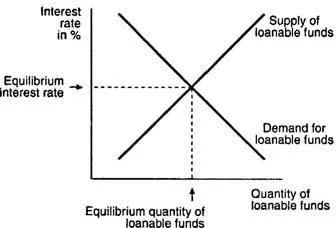
A common mistake students make is to try to use the market for loanable funds graph to try to figure out what the interest rate will be in the short run. That doesn’t work well. Although technically possible, it would be confusing, since how far the economy is above or below the natural level of output has a big effect on both the supply and the demand for loanable funds that using the market for loan. To understand the short-run natural interest rate, it is much better to use a graph designed for that purpose–a graph that focuses on how the short-run natural interest rate is determined by the demand for capital to use in production and by monetary policy.

The Short-Run Natural Interest Rate

Above, I defined the short-run natural interest rate as the "rental rate of capital, net of depreciation,“ or "net rental rate,” for short. What does this mean?

Renting Capital. First, to understand what it means to rent capital, think of those ubiquitous office parks. If the capital a company or other firm needs is an office to work in, it can rent one in an office park like this:

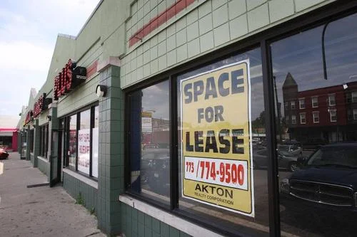
In retail, the capital a firm needs to rent might be retail space in a strip mall:

If a firm is in construction or landscaping, the capital it needs might be a bulldozer, which it can rent from the Cat Rental Store, among other places.

Of course, sometimes a firm needs specialized machine that it has to buy, because those machines are hard to rent. In that case, let me treat it as two different firms: one that buys the specialized machine and puts it out for rent, and another firm that rents the machine. The same trick works for a specialized building that is hard to rent, such as a factory designed for a particular type of manufacturing. When firms that own buildings or machinery are short of cash, sometimes they separate themselves into exactly these two pieces, and sell the piece that owns the specialized buildings or machines so the other piece of the firm can get the cash from the sale of those buildings or machines, while still being able to use those buildings and machines by paying to rent them.

The (Gross) Rental Rate. I will call the gross rental rate simply “the rental rate." The rental rate is equal to the rent paid on a building or piece of equipment divided by the purchase price of that building or piece of equipment. Because this is one price (expressed for example in dollars per year) divided by another price (dollars per machine), the rental rate is a real rate–that is, it does not need to be adjusted for inflation. The rental rate is usually expressed in percent per year, meaning the percent of the purchase price that has to be paid every year in order to rent the machine.

The Net Rental Rate. It is useful to adjust the rental rate for depreciation, however. The paradigmatic case of depreciation is physical depreciation: a machine or building wearing out. More generally, a machine or building might become obsolete or start to look worse in comparison with newer machines. I am going to treat obsolescence as a form of depreciation. Obsolescence shows up in the price of new machines or buildings of that type falling relative to the prices of other goods in the economy. There are other things that can affect the prices of machines and buildings that will matter for the story below, but the rate of physical depreciation and the rate of obsolescence measured by declines in the real price of new machines and buildings of given types at the long-run trend rate are the two to subtract from the rental rate to get the net rental rate.

The Determination of Physical Investment

Physical investment is the creation of new capital–such as machines, buildings, software, etc.–that can be used as factors of production to help produce goods and services. Notice that I am using the phrase "physical investment” to distinguish what I am talking about from “financial investment.” So in this case, at some violence to the English language, I include writing new software in “physical investment."

The amount of physical investment is determined by the costs and benefits of creating new machines, buildings, software, etc. now instead of later. Say we are talking about whether to create or purchase a building or machine now, or a year from now. The benefit of creating a new building or machine a year earlier is the rent that building or machine could earn in that year. In the absence of capital and investment adjustment costs (to which I return below), the cost of creating a new building or machine a year earlier is

interest on the amount paid to create or purchase the building or machine.
physical depreciation
obsolescence

Dividing all of the costs and benefits by the amount paid to create or purchase the building or machine, the costs and benefits per dollar spent on the machine are

benefit relative to amount spent = rental rate

cost relative to amount spent = real interest rate + physical depreciation rate + obsolescence rate

The reason it is the real interest rate in the cost relative to amount spent is because the obsolescence rate is being measured in terms of a real price decline.

In the absence of capital and investment adjustment costs, the rule for physical investment is:

If the rental rate is less than (the real interest rate + physical depreciation rate + obsolescence rate), invest later.
If the rental rate is more than (the real interest rate + physical depreciation rate + obsolescence rate), invest now.

If I move the physical depreciation rate and the obsolescence rate to the other side of the comparison, I can say the same thing this way:

If the rental rate net of net of physical depreciation and obsolescence is below the real interest rate, invest later.
If the rental rate net of physical depreciation and obsolescence is above the real interest rate, invest now.

Or more concisely:

If the net rental rate is less than the real interest rate, invest later.
If the net rental rate is more than the real interest rate, invest now.

Finally, using the definition of the short-run natural interest rate as the net rental rate and flipping the order, I can describe the rule for investment this way:

If the real interest rate is above the short-run natural interest rate (the net rental rate), invest later.
If the real interest rate is below the short-run natural interest rate (the net rental rate), invest now.

The Determination of the Short-Run Natural Interest Rate: Capital Equilibrium (KE) and Monetary Policy (MP)

Susanto Basu and I have a rough working paper on the determination of the short-run natural interest rate and about very-short-run movements of the actual interest rate in relation to the short-run natural interest rate:

"Investment Planning Costs and the Effects of Fiscal and Monetary Policy” by Susanto Basu and Miles Kimball.

We also have a set of slides to go along with the paper:

Slides for “Investment Planning Costs and the Effects of Fiscal and Monetary Policy” by Susanto Basu and Miles Kimball.

The short-run natural interest rate is determined by (a) equilibrium in the rental market for capital and (b) monetary policy.

Capital Equilibrium (KE): Supply and Demand for Capital to Rent

The Supply of Capital to Rent: The supply of capital to rent cannot change very fast. It takes time to create enough new machines, buildings, software, etc. through physical investment to affect the total amount of capital available to rent in any significant way. Wikipedia has an excellent article “Stock and flow” about this relationship between capital and physical investment. The canonical illustration is this picture of a bathtub:

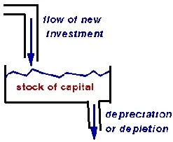
Turning the tap on full blast might double the flow of water, but it will still take time for that flow to significantly affect the overall level of water in the tub. Similarly, turning investment on full blast may double the rate of physical investment creating new machines, buildings, software, etc., but it will still take time to significantly affect the overall amount of capital that exists in the form of machines, buildings, software, etc.

The Demand for Capital to Rent: The most important thing to understand about the demand for capital to rent is that it is higher in booms than in recessions. The more goods and services people want to buy, the more capital firms will want to rent at any given rental price in order to produce those goods and services. Ask any business person who has been involved in a decision to buy capital and they will tell you that they are more eager to get hold of capital to use when business is good than when business is bad.

The way I think of why the demand for capital to rent is higher in a boom than in a recession is this:

Since profit is revenue minus cost, whatever amount of output a profit-maximizing firm decides to produce to sell or inventory, it should try to produce that amount of output at the lowest possible cost.
In a boom a firm will produce more output than in a recession (other things equal).
Since the stock of capital can’t change very fast, when the economy booms and firms add worker hours, a typical firm will not have as much capital per unit of labor as before.
The more the economy booms, the higher wages will be. (How much depends on whether wages are sticky or not. On sticky wages, if you are prepared for a hardcore economics post, see “Sticky Prices vs. Sticky Wages: A Debate Between Miles Kimball and Matthew Rognlie.”)
What is true of labor is also true for intermediate goods firms use as material inputs into production: when the economy booms and firms buy more materials to use, a typical firm will not have as much capital per unit of material inputs as before.
Also, the more the economy booms, the higher the price of intermediate goods used as material inputs will be. (How much depends on whether the prices of the material inputs are sticky or not.)
When the typical firm has less capital per unit of other inputs, it will be more eager to rent capital at any given rental price.
If the firm is employing more labor and using more of other inputs despite wages and other input prices being high, it will be especially eager to rent additional capital at a given rental price, since capital then is relatively cheaper than other inputs.

The math behind this story is in the Basu-Kimball paper “Investment Planning Costs and the Effects of Fiscal and Monetary Policy.” There, although it is not needed to get these results, for simplicity we use the fact that for Cobb-Douglas production functions, the ratio of how much a cost-minimizing firm spends on labor and on capital is fixed. (See the relatively hardcore post “The Shape of Production: Charles Cobb’s and Paul Douglas’s Boon to Economics.”) Using the letters

R for the the rental rate,
K for the amount of capital,
W for the wage, and
L for the amount of total worker hours,

that means

RK = constant * WL.

Dividing both sides of this equation gives an equation for the rental rate:

R = constant * WL/K.

Since the total amount of capital K in the economy can’t change very fast, the total amount of capital in the typical firm also can’t change fast, so increases in wages W and total worker hours will push up the rental rate. And the net rental rate will parallel the overall gross rental rate very closely.

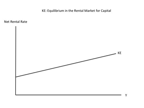
The KE Curve. With the supply of capital relatively fixed (or technically “quasi-fixed”) at any moment in time, a higher demand for capital means a higher equilibrium rental rate in the market for renting capital. How much a typical firm chooses to produce is closely related to how much output the economy as a whole produces. (Indeed, the amount firms produce must add up to the amount of output in the economy as a whole.) So the overall gross rental rate–and the net rental rate–will be increasing in the amount of output the economy as a whole produces. And of course, the amount of output the economy as a whole produces is GDP, for which we will use the single letter y. Thus, the graph below, which has GDP on the horizontal axis, and like the graph at the top of this post, shows an upward slope for the KE curve:

The KE Curve vs. the IS Curve. The IS curve has no microfoundations. The KE curve does. That is, I just explained where the KE curve comes from. The explanations of where the IS curve comes from are either incoherent, or really imply something very different from the IS curve taught in introductory and intermediate macroeconomics classes. Let me critique several ways people convince themselves the IS curve is OK. (Don’t worry if you haven’t heard of some of the interpretations I am critiquing.)

The consumption Euler equation as an IS curve: The consumption Euler equation is an equation about changes rather than levels. Much more seriously, the consumption Euler equation acts like some sort of IS curve only in models that don’t have investment or other durables. Investment and other durables play such a big role in economic fluctuations that it It is hard to take a model of economic fluctuations that leaves out investment and other durables seriously. Bob Barsky, Chris House and I show how big a difference it makes to sticky price models to bring in investment or other durables goods in our paper “Sticky-Price Models and Durables Goods,” which appears in the American Economic Review.
Q-theory as a foundation for the IS curve: Like the consumption Euler equation, Q-theory yields a dynamic equation, instead of one that can be drawn as a simple curve with output on the horizontal axis and the real interest rate on the vertical axis. Q-theory says that firms might invest now even if the interest rate is above the net rental rate as long as the level of investment is increasing over time. The reason is that it will be harder to invest later when investment is proceeding faster, so it could make sense to get a jump on things and invest now. On the other hand, firms might delay investment even if the interest rate is below the net rental rate if the level of investment is decreasing over time. The reasons is that it will be easier to invest later when investment is proceeding more slowly, so it could make sense to wait until later when investment can be done in a more leisurely way. Suppose that we show the short-run equilibrium in terms of output and the real interest rate (rather than the net rental rate) and that higher investment is associated with higher GDP, as is usually the case. Then in relation to the KE curve, what Q-theory means is that the short-run equilibrium can be above the KE curve if that equilibrium point is moving to the right (GDP is increasing along with investment), while the short-run equilibrium can be below the KE curve if the equilibrium point is moving to the left (GDP is decreasing along with investment). But the slower the equilibrium point is moving, the closer it has to be to the KE curve. So when the “short-run” lasts a long time, as it has in the last five years since the bankruptcy of Lehman Brothers, the short-run equilibrium needs to be quite close to the KE curve. I discuss how the speed with which the economy is headed toward the medium-run equilibrium affects what can be gotten out of the Q-theory story in “The Quantitative Analytics of the Basic Neomonetarist Model.”
Heterogeneity of investment projects as a foundation for the IS curve: Heterogeneous investment projects, with some being able to clear a high interest-rate hurdle and some only being able to clear a low-interest-rate hurdle is the traditional story for the IS curve. This is actually a very interesting story, and one my coauthors Bob Barsky, Rudi Bachmann and I have been thinking about for a project in the works, but it actually points to something much more complex than an IS curve. For example, if potential investment projects are heterogeneous, then in general, one needs to keep track of how many are still available of each type. In any case, there is nothing simple about such a story.

The MP Curve. Central banks periodically meet to determine the interest rate they will set. The rate they set is a nominal interest rate, where “nominal” just means it is the interest rate that non-economists think of. The real interest rate is the nominal interest rate minus expected inflation. Inflation expectations tend to change quite slowly and sluggishly, so the nominal interest rate the central bank chooses determines the real interest rate in the short run and the very short run. Central banks ordinarily raise their interest rate target when the economy is booming and lower it when the economy is in recession, so the interest rate (both nominal and real) will be upward sloping in output. Indeed, in order to make the economy stable, the central bank should make sure that the real interest rate goes up faster with output than the net rental rate does, so that, going from left to right, the MP curve showing how the central banks target interest rate depends on output cuts the KE curve from below, as shown in the complete KE-MP diagram:

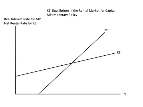
In the KE-MP model, the intersection of the KE and MP curves is the short-run equilibrium of the economy. In short-run equilibrium, the real interest rate equals the net rental rate, or equivalently, the real interest rate equals the short-run natural interest rate.

The Ultra Short Run

What brings the economy to short-run equilibrium is the adjustment of investment based on the gap between the net rental rate determined by the KE (capital rental market equilibrium) curve and the real interest rate determined by the MP (monetary policy) curve. But it takes time for firms to adjust their investment plans. Indeed, the level of investment is unlikely to adjust much faster than existing investment projects are completed and a new round of investment projects is started, as Susanto Basu and I discuss in “Investment Planning Costs and the Effects of Fiscal and Monetary Policy.” In the meanwhile, before investment has had time to full adjust, output can be away from its short-run equilibrium level, and the interest rate determined by the MP curve can be different from the net rental rate determined by the KE curve.

For example, suppose that the economy starts out in short-run equilibrium, but then the central bank decides to make a change in the interest rate change for some reason other than a change in the level of output. Since output is unchanged, the change in the interest rate corresponds in the KE-MP model to a shift in the MP curve. The graph below, taken from Slides for “Investment Planning Costs and the Effects of Fiscal and Monetary Policy,” shows the effects of a monetary expansion.

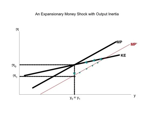
The movement up along the MP’ curve reflects the ultra-short-run adjustment of investment to get to the new short-run equilibrium–a process that might take about 9 months. The movement back along the unchanging KE curve reflects the short-run adjustment of prices to get back to the original (and almost unchanged) medium-run equilibrium. Since the real interest rate is on the axis, the point representing first ultra-short-run equilibrium, and then short-run equilibrium, is always on the MP curve. (The graph does not show the gradual shift of the MP curve back to return the economy to the medium-run equilibrium. One way for that adjustment of the MP curve to happen is if there is some nominal anchor in the monetary policy rule so that the level of prices matters for monetary policy, not just the rate of change of prices.)

Why It Matters: Remarks About the KE-MP Model

The reason I wrote this post is because many people don’t seem to understand that low levels of output lower the net rental rate and therefore lower the short-run natural interest rate. Leaving aside other shocks to the economy, monetary policy will not tend to increase output above its current level unless the interest rate is set below the short-run natural interest rate. That means that the deeper the recession an economy is in, the lower a central bank needs to push interest rates in order to stimulate the economy. In the Q-theory modification of the KE-MP model, the belief that the economy is going to recover fast could generate extra investment even if interest rates are somewhat higher, but when such confidence is lacking, the remedy is to push interest rates below the net rental rate that is the short-run natural interest rate.
As discussed in “Investment Planning Costs and the Effects of Fiscal and Monetary Policy” and the Slides for “Investment Planning Costs and the Effects of Fiscal and Monetary Policy,” fiscal policy and technology shocks have counterintuitive effects on the KE curve. This is grist for another post. Also grist for another post is the way a version of the Keynesian Cross comes into its own in the ultra short run, but only during the 9 months or so of the ultra short run.
If a country makes the mistake of having a paper currency policy that prevents it from lowering the nominal interest rate below zero, then the MP curve has to flatten out somewhere to the left. (The zero lower bound on the nominal interest rate puts a bound of minus expected inflation on the real interest rate. That makes the floor on the real interest rate higher the lower inflation is.) The lower bound on the MP curve might then make it hard to get the interest rate below the net rental rate (a.k.a. the short-run natural interest rate). In my view, this is what causes depressions. QE can help, but is much less powerful than simply changing the paper currency policy so that the nominal interest rate can be lowered below the short-run natural interest rate, however low the recession has pushed that short-run natural interest rate. (See the links in my post “Electronic Money, the Powerpoint File” and all of my posts on my electronic money sub-blog.)