On the Great Recession
I am honored to have David Andolfatto discuss my proposal for eliminating the zero lower bound in his post “Are negative interest rates really the solution?” David asks what model I have in mind when I write, for example, in “America’s Big Monetary Policy Mistake: How Negative Interest Rates Could Have Stopped the Great Recession in Its Tracks,"
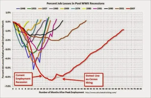
Even without the ZLB [the zero lower bound on nominal interest rates], there would have been some hit from the financial crisis that ensued with the bankruptcy of Lehman Brothers on Sept. 15, 2008, but negative interest rates in the neighborhood of 4% below zero would have brought robust recovery by the end of 2009.
This post gives that model.
One thing I will not try to do in this post is to talk about how we have actually been crawling out of the hole left by the great recession using the low-power, but not powerless tool of quantitative easing. Among instruments of monetary policy, this post considers only the current short-run safe interest rate. (I discuss some of the downsides of quantitative easing relative to negative interest rates in my ”Breaking Through the Zero Lower Bound" Powerpoint file.)
Related Work
It is a model that I have taught in my advanced undergraduate course “Business Cycles” since the mid-90’s (see scans of student notes for two different years 1, 2), building on my academic papers
Are Technology Improvements Contractionary? (with Susanto Basu and John Fernald)
Sector-Specific Technology Shocks (with Susanto Basu, John Fernald and Jonas Fisher)
Investment Planning Costs and the Effects of Fiscal and Monetary Policy (with Susanto Basu; see slides here)
(My “Business Cycles” course is Economics 418 at the University of Michigan. Masao Ogaki has also arranged for me to teach it at Keio University in Tokyo, in August 2014.)
I am currently working on a formal treatment of the kind of issues I will address here with Bob Barsky and Rudi Bachmann. Blogging has brought home to me the policy importance of pushing that paper through to completion. We do not have a full draft yet, but if you want to see the kind of model it is, here is a mathematical appendix I put together early on in our process of writing that paper.
But to understand what I am going to say, you don’t need to read the academic papers I flag above. The only indispensable prerequisite for understanding what I am going to say beyond a general background in economics is to read my post “The Medium-Run Natural Interest Rate and the Short-Run Natural Interest Rate,” where I discuss why I reject the IS-LM model on theoretical grounds, using instead the soundly micro-founded KE-MP model.
The Argument for Sticky Prices, Sticky Wages or Sticky Information or Sticky Information Processing Relevant to Prices and Wages
I am claiming that the KE-MP model is soundly “micro-founded,” but “micro-founded” is of course always a matter of degree. The Arrow-Debreu model is not fully micro-founded because it does not explain how the contracts at its heart are enforced! In the case of the KE-MP model, the place where the micro-foundations do not go as deep as one might wish is in explaining why prices are determined in the way they are. I consider the evidence of substantial monetary nonneutrality (from Friedman and Schwartz, from Romer and Romer, from vector auto-regressions, from the experience of central bankers even after allowing for some of the likely psychological biases, etc.) very persuasive. Despite many attempts, models without sticky prices, sticky wages or some kind of sticky information or sticky information processing relevant for prices and wages have not been very successful at explaining substantial monetary nonneutrality. (In saying this, I am leaving aside models that, in their totally real versions, have multiple equilibria; it is of course easy to have nominal things help select among multiple real equilibria.) Thus, regardless of the qualms one might have about why prices might be sticky (or wages, or information relevant to prices and wages), it is appropriate to assume something that is the moral equivalent of sticky prices in the broad sense.
Many people do not realize that there is another very powerful strand of evidence for something like sticky prices: the observed response of the economy to technology shocks. In “Are Technology Improvements Contractionary?”Susanto Basu, John Fernald and I make a careful, extensive, and I believe persuasive, argument that the observed response of the economy to technology shocks is very hard to square empirically with models that lack something like sticky prices, sticky wages or sticky information or sticky information processing relevant to prices and wages. I have been disappointed in the years since it was published that this aspect of our paper–this argument for sticky prices or the like–has had as little influence as it has. (Of the many citations the paper has, the bulk appear to be from economists who are simply eager to use our measure of technology shocks.)
As for the empirical evidence behind "Are Technology Improvements Contractionary?“, it is nice to know that our evidence based on purifying Solow Residuals of variable capital and labor utilization and increasing returns to scale to identify technology shocks is backed up by the very different methodology of structural vector autoregressions of aggregate hours and output, beginning especially with Jordi Gali’s paper ”Technology, Employment, and the Business Cycle: Do Technology Shocks Explain Aggregate Fluctuations?“ (which was actually contemporaneous with our work in ”Are Technology Improvements Contractionary?“ in its inception, but was completed much more quickly than our paper), and ably defended by John Fernald in his paper Trend Breaks, Long-Run Restrictions, and Contractionary Technology Improvements.
One of the important contributions of ”Are Technology Improvements Contractionary?“ is to focus on the evidence that technology improvements are contractionary for business investment as well as for labor hours. That evidence for a contractionary effect on business investment of immediate permanent technology shocks, is actually much more decisive as evidence for something like sticky prices than the evidence of a contractionary effect on hours. (Note that if technology improvements are anticipated in advance, in a real business cycle model they should make both investment and hours increase at the moment when the technology actually improves. But both investment and hours decline when the technology is observed to improve.)
I should mention in passing that the response of the economy to technology shocks only provides evidence for sticky prices because the monetary policy response to technology shocks is suboptimal. An optimal monetary policy response to technology shocks should strive to make the economy behave like the real business cycle model corresponding to perfectly flexible prices. (In my column "Show Me the Money” I discuss the importance of monetary policy responses to tax policy changes as well as technology shocks.)
Sluggish Inflation
In the graphs I present below, I will treat inflation as being relatively sticky and unchanging. I was clued into the importance of sluggishly changing inflation by Michael Kiley’s job talk at the University of Michigan in 1995 and presented my own (never published) model to generate that kind of behavior at a seminar at Harvard in May, 2000. But given the premium on actually publishing things in academic journals, I gave this account of those ideas in my post “Trillions and Trillions: Getting Used to Balance Sheet Monetary Policy”:
I take the idea that inflation adjusts gradually from my main graduate school advisor Greg Mankiw, one of the most eminent New Keynesians: both from his textbook where he gives his view of the facts and from his theoretical 2002 paper with Ricardo Reis trying to explain those facts: “Sticky Information Versus Sticky Prices: A Proposal to Replace the New Keynesian Phillips Curve.”Michael Kiley anticipated Mankiw and Reis in his 1995 job market paper. He used the nice phrase “sluggish inflation” to describe what he was explaining with his model.
The thing I emphasize to my graduate students is that if inflation is sticky, as distinct from the price level being sticky, that some kind of imperfect information processing must be involved. Why? Let’s think of a continuous-time model–or it is good enough to think of a model with 365 periods per year–for clarity. Inflation yesterday was generated by the firms that changed their prices yesterday. But with staggered price setting, the firms that were changing their price yesterday are different firms than the one that are changing their prices today. So, other than having a similar information environment, there is nothing connecting inflation yesterday to inflation today. If firms are optimally using all available information, and something big happens between yesterday and today, then inflation should jump, since the optimal price to change to today should generally be different than the optimal price to change to yesterday. (I am assuming that the old price firms are changing from is changing gradually at that juncture.) To make inflation not jump when something important happens requires firms today somehow not fully using that new information. That is, there has to be some form of imperfect information processing. Mankiw and Reis model the imperfect information processing as firms being asleep relative to new information and making up price changes based on old information much of the time, then periodically updating the information set they are using in full
The key evidence for sluggish inflation is how costly it seems to be to reduce inflation. Paul Krugman gives a nice (though as usual, combatively framed) description of the relevant historical episode in his very interesting post “Fighting the Last Macro War?”:
So, what were the macro wars of the last few decades? First there was stagflation — and that did indeed knock Keynesians back for a while, even as it gave freshwater macro some credibility. As I’ve already indicated, the freshwater guys then stopped there. And I mean really, really stopped there: in many ways they seem to be forever living in 1979.
In particular, they never reacted at all to the second macro war, the disinflation of the 1980s. The point there was that disinflation was very costly, with protracted high unemployment — which shouldn’t have happened if freshwater macro were at all right. This reality, as much as clever new models, drove the Keynesian revival …
What Paul doesn’t say there, but I think would agree with, is that costly disinflation is not only evidence for monetary nonneutrality, but also evidence against something as simple as the usual Calvo model of price setting, which has sticky prices, but jumping inflation. Indeed, Larry Ball among others pointed out that the Calvo model implies that disinflation brought on by a gradual reduction in the growth rate of the money supply should cause a boom if price setting were as in the usual Calvo model of price setting.
In any case, though the usual Calvo model might be OK for some pedagogical purposes, it is seriously flawed as a representation of reality in any context in which it might matter whether inflation is sluggish or not. For a recent, brief discussion of evidence for sluggish inflation in the context of the Great Recession, see Bob Hall’s strong words in “The Routes into and out of the Zero Lower Bound”:
The historical pattern is that a rise in unemployment generates a transitory decline in inflation, but the rise wears off quite quickly, and an extended period of high unemployment|as in the U.S. since 2007 has no effect on inflation.
(Note: I am not persuaded by Bob Hall’s story for why inflation has not fallen faster during the Great Recession.)
The KE-MP Model
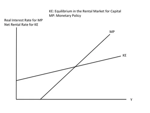
I build the KE-MP model in “The Medium-Run Natural Interest Rate and the Short-Run Natural Interest Rate.” So far, this is the version without a zero lower bound.
The MP curve is simply the monetary policy rule, which says that at its regular meetings (every six weeks or so for the Fed) the monetary policy committee will raise the target interest rate if output is higher than at the last meeting and lower the target interest rate the Fed will raise the target interest rate if output is lower than at the last meeting.
The KE curve shows what happens as a result of equilibrium in the capital rental market. The key point is that firms will be willing to pay more to rent capital when the economy is in a boom than when the economy is in recession. Therefore, the rental rate for capital is an upward-sloping function of output. (As I discuss in The Quantitative Analytics of the Basic Neomonetarist Model, even adding a Q-theory-type investment-smoothing motive modifies this story less and less the longer-lasting a recession is. All the ins and outs of that kind of modification are one of the key issues addressed by the paper I am working on with Bob Barsky and Rudi Bachmann.)
To begin with, think of short-run equilibrium as requiring that the short-term interest rate equal the rental rate net of depreciation. The reason is one that goes back to Dale Jorgenson: if the net rental rate is less than the real interest rate, then a firm would be better off waiting until later to invest. So it won’t invest now. If the net rental rate is higher than the real interest rate, then a firm should be eager to invest now (as long as a generic investment project meets the longer-run positive present-discounted value test–something that is guaranteed unless interest rates are expected to be above the net rental rate in the future).
To give my view of the Great Recession, in addition to imposing the zero lower bound on the MP curve, I need to add one important wrinkle to the KE curve–a risk premium between the net rental rate and the safe interest rate. Because building a building, buying equipment or writing software or uncertain value is risky, the net rental rate actually needs to be higher than the safe short-term interest rate for a firm to invest now instead of later. Given that, I want the KE curve to represent not the net rental rate, but the risk-adjusted net rental rate–that is, the safe interest rate that is just low enough that, given the risk premium, would make firms indifferent between investing now and investing later. In many discussions with Tomas Hirst (see for example “Doubting Tomas: Electronic Money in an Open Economy with Wounded Banks”), he writes as if the relevant risk premium is infinite. In my model, it isn’t. And I don’t think the risk premium is infinite in the world either. There is some real interest rate low enough that firms will not want to delay investment until later. Nevertheless, the risk premium tends to (a) be lower in good times than in bad times, lending a higher slope to the risk-adjusted KE curve, and (b) to change for reasons other than the current level of output, causing shifts in the risk-adjusted KE curve.
The Risk-Adjusted KE Curve
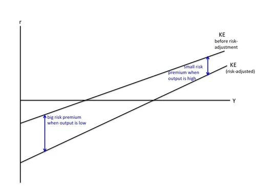
To see why the relationship of the risk premium to the output gap makes the risk-adjusted KE curve more strongly upward-sloping, note that
at low levels of output (on the left in the graph just above), the risk-premium pushes the risk-adjusted KE curve a long way below the before-risk-adjustment KE curve
at high levels of output (on the right in the graph just above), the risk-premium pushes the risk-adjusted KE curve only a modest distance below the before-risk-adjustment KE curve.
From here on, the curve labeled “KE” will always be the risk-adjusted KE curve: the locus of safe short term rates that makes a typical firm indifferent between investing now and investing later on a generic investment project.
Imposing the Zero Lower Bound on the MP Curve and Accounting for Sources of Aggregate Demand Other than Generic Investment Projects
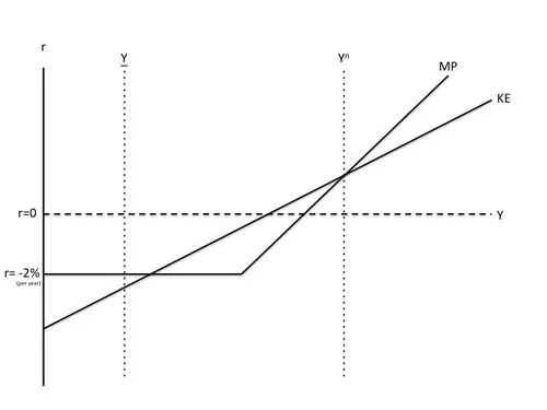
I have written a lot about the zero lower bound and how to eliminate it. See my reader’s guide “How and Why to Eliminate the Zero Lower Bound" Graphically, since the real interest rate is the nominal interest rate minus expected inflation, if inflation is steady at 2% per year (the long-run inflation target for the Fed, the European Central Bank and the Bank of England, and currently the fond wish of the Bank of Japan), then the zero lower bound on the nominal interest imposes a lower bound of -2% per year on the real interest rate.
In addition to the KE and MP curves that govern generic investment, there is one other key element of the graph above: the level of output when generic investment is zero: Y(read "Y underbar”). When generic investment is zero, aggregate demand is composed of consumption, government purchases, net exports, and investment from special investment opportunities.
For simplicity I am treating the special investment opportunities as so good that they will be pursued regardless of any changes in the risk-adjusted net rental rate or the real interest rate during this episode. Government purchases are exogenous. Consumption is determined by people’s views about the post-recession future according to the permanent income hypothesis. (The elasticity of intertemporal substitution in the model is low enough that interest rate effects on consumption can be ignored if interest rate fluctuations are short-lived.) If you want to think of this as a simplified model of the world economy, then net exports are zero. Alternatively, think of other country’s central banks matching most interest rate moves for the safe short-term rate, so that there is very little change in international capital flows or the closely linked value of net exports.
What is a generic investment project in the real world? I suspect it is building a house. Note that rental rates for housing, like rental rates for factories and machines, are likely to be higher in good times than in bad times. So there would still be an upward-sloping KE curve if house construction is the main component of “generic investment.” For this to work, it turns out to be crucial that house prices are sticky, even from at the moment construction commences on a house–as Bob Barsky, Chris House and I argue in our paper “Sticky Price Models and Durable Goods.” Thinking about it from the standpoint of theory, it is quite mysterious to me why house prices would be sticky, yet it seems consistent with the data to say that they are. If the typical generic investment project is building a house, then a key transmission mechanism for a typical recessions would be a partial or total shutdown of house construction.
The 3 Equilibria in Normal Times
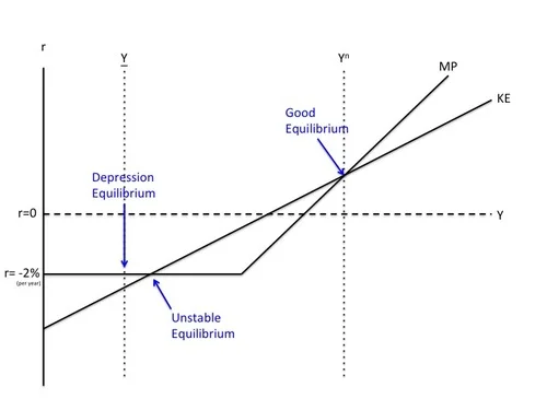
I am not in general a fan of multiple equilibrium models. Here, except for the zero lower bound, there would be only a single stable equilibrium. But the zero lower bound often creates two additional equilibrium. The rightmost intersection between KE and MP above is what I will call “the normal equilibrium” or “the good equilibrium.” (In the graph I have drawn the good equilibrium at the natural level of output Yn, which is where it will be in medium-run equilibrium.) The good equilibrium is the equilibrium that would remain in the absence of the zero lower bound (unless monetary policy were intentionally so tight as to push output down to Y). The good equilibrium is stable because
if output gets a little above that level, the central bank will raise the real interest rate above the risk-adjusted net rental rate, causing firms to start delaying investment projects that are not already underway, leading to a gradual decline in investment as investment projects already underway gradually get completed. That gradual downward adjustment of investment takes about nine months, and brings output back down to the short-run equilibrium level at the intersection of KE and MP. (See “Investment Planning Costs and the Effects of Fiscal and Monetary Policy" for the background for this gradual investment adjustment process.)
If output gets a little below that level, the central bank will lower the real interest rate below the risk-adjusted net rental rate, and firms will then be eager to do generic investment projects immediately–or as soon as they can be planned out. The extra aggregate demand from these additional investment projects will gradually cause output to rise back to the short-run equilibrium level at the intersection of KE and MP.
Notice that in this story, it is crucial for stability that the central bank raise its target interest more with changes in output than the rate at which the risk-adjusted net rental rate changes with changes in output. (This is a very different kind of stability issue than what is often emphasized in monetary models.) Not making the target interest rate go up strongly enough with output would lead to instability. And indeed, the intersection of the zero-lower-bound portion of the MP curve with the KE curve is an unstable equilibrium. Let me justify the label of "unstable equilibrium” that I have given to that point.
To the right of the intersection where the KE curve cuts the horizontal MP curve from below, the risk-adjusted net rental rate is above the real interest rate, which encourages more investment and raises leads to even higher output, leading ultimately to the normal equilibrium.
To the left of that intersection where the KE curve cuts the horizontal MP curve from below, the risk adjusted net rental rate is below the real interest rate, making firms want to delay all generic investment projects (according to Dale Jorgenson’s logic), leading to a decline in investment as projects already underway are completed, and a corresponding decline in output, which would only end when generic investment has been completely shut down, bringing output down to Y.
Finally at Y, there is a stable “depression equilibrium.” At that point, the risk-adjusted net rental rate is below the real interest rate, so firms want to delay all generic investment projects. Even if something made output go up a tad, the risk-adjusted net rental rate would still be strictly below the real interest rate, so firms would still want to delay all generic investment projects. With all generic investment projects delayed, output will be stuck at Y, which is the level of output that can be supported by aggregate demand from consumption, government purchases, net exports and special investment projects.
An Increase in the Risk Premium Leads to a Collapse of Generic Investment
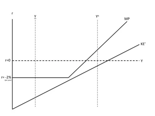
In my model, there is no confidence fairy. Equilibrium selection is simple: once in one of the two stable equilibria, the economy stays in that equilibrium (with what ever adjustments occur to that equilibrium), unless the time comes when that equilibrium ceases to exist. The trouble is that, for a while at the end of 2008 and early 2009, the good equilibrium didcease to exist. For reasons that we understand at the same level that non-economists do, but do not understand at a deep theoretical level, the risk premium increased, and the KE curve therefore shifted down. Indeed, my view is that it shifted down enough that the the panic KE curve, labeled KE’, was everywhere below the MP curve, given the constraint imposed by the zero lower bound. With risk-adjusted net rental rate for generic investment projects everywhere below the real interest rate, generic investment began shutting down, and the economy headed toward the depression equilibrium.
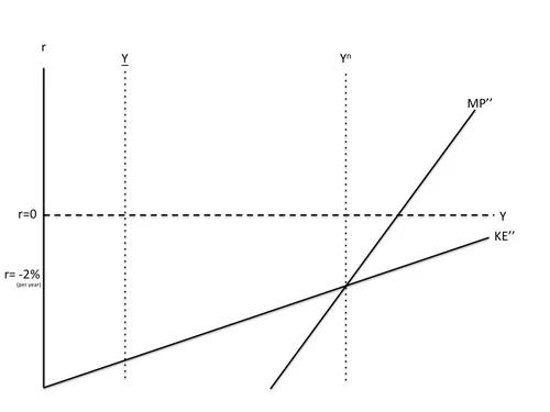
The Effects of Some Monetary Easing and Some Reduction in the Risk Premium, Subject to the Zero Lower Bound

Just above, I have drawn KE after some success of efforts to reduce the risk premium (labeling it KE’’) and MP after some monetary easing (labeling it MP’), but still subject to the zero lower bound. If all of this could have been done quickly enough, it might have been possible to get the risk-adjusted net rental rate above the real interest rate while the level of output was still above the unstable equilibrium at the intersection of the zero lower bound with the somewhat restored KE curve. But by the time these steps were completed, output was already below the level at the unstable equilibrium. Thus, the risk-adjusted net rental rate was already below the real interest rate, and the zero lower bound prevented the real interest rate falling enough to change that inequality. So the economy continued heading toward the depression equilibrium.
Eliminating the Zero Lower Bound and Going to Negative Interest Rates Leads to Recovery by the End of 2009 (What Could Have Been)
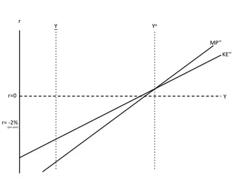
If there had been no zero lower bound, a straightforward shift downward in the MP curve to compensate for the increase in the risk premium could have kept the short-run equilibrium at the natural level of output. Here I have drawn a KE’’ curve a little higher than the KE’ curve was in order to represent some success of efforts to bring the risk premium back down, but that is not essential. However much the KE curve goes down, it is possible to shift the MP curve down just as much.
Of course, if the risk premium were going to stay high for years and years, that would have some effect on the natural level of output, but other than the delay condition highlighted in the KE-MP graph, it is only the time integral of the risk premium that matters. So a year or two of an elevated risk premium probably would not have a big effect on the natural level of output. And along with the bailouts that actually took place, and reasonable macroprudential efforts to avoid a repeat of the financial crisis, the economic recovery from effective monetary policy–unhindered by the zero lower bound–would probably have kept the effects on the risk premium quite reasonable in duration.
Let me make a few more points here. First, the reason I said the recession would be over by the end of 2009 is that it takes about 9 months for investment to adjust to changes in monetary policy. Second, there is no need to posit any technology shock to explain the Great Recession. Risk premia shocks indeed real shocks, but they differ from technology shocks in mattering for the natural level of output (the medium-run equilibrium) only in proportion to how long they are going to last. By contrast, as is well known from the Real Business Cycle literature, even a short-lived technology shock, if there were such a thing, would have a very powerful effect on the medium-run equilibrium. (In a real business cycle model, among things easy to draw in a phase diagram, a risk premium shock is more like a temporary shock to the utility discount rate.) Third, it is good to check in the graph just above that there is only one stable equilibrium; with the appropriate shift in the MP curve shown, that equilibrium is at the (mostly unchanged) natural level of output. Thus, the recession has been ended with more or less full recovery. Finally, if the central bank doesn’t go to negative interest rates until later on, the capital stock is likely to have declined somewhat, reducing the natural level of output.
Bonus: Fiscal Policy in the KE-MP Model
I am done with my main message. And I consider fiscal policy markedly inferior as a way to deal with the kind of thing we faced in the last few years. But it is of some interest to see what the model here has to say about changes in government purchases. The first thing to say is that at the good equilibrium, increases in government purchases crowd out generic investment 1 for 1 in the short-run equilibrium. Because investment plans take time to adjust, speedy changes in government purchases could have an effect on the ultra-short-run equilibrium for about 9 months (as discussed in “Investment Planning Costs and the Effects of Fiscal and Monetary Policy”), but changes in government purchases that took just as long to plan would have no effect on output. (It is possible to get some longer-lasting effects of government purchases on output, but it requires putting more barriers in the way of adjustments in generic investment than the KE-MP model has.)
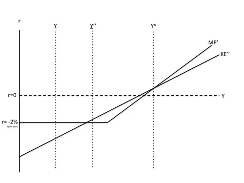
The Effects of an Increase in Government Purchases at the Zero Lower Bound
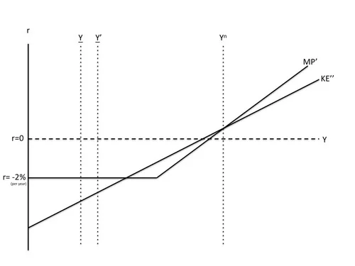
Once the economy is in the depression equilibrium, an increase in government purchases cannot crowd out generic investment because generic investment is already zero. Thus, an increase in government purchases raises Y to Y’. For modest increases in government purchases (say, like the actual stimulus package), though this improves the depression equilibrium, it does not get the economy out of the depression equilibrium. But given some success at reducing the risk premium and loosening of monetary policy where possible above the zero lower bound, if the increase in government purchases were large enough (say three times as big as the actual stimulus package), it might push output to Y’’, as shown below, a higher level of output than the unstable equilibrium, bringing the risk-adjusted net rental rate above the -2% per year real rate at the zero lower bound, and reignite generic investment. (See below.) Note that there is critical level of government purchases that does this, and a discontinuity in the effects of government purchases at that level.
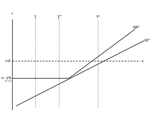
The graph below shows a situation where efforts to bring the risk premium back down have been less successful. Here the triple-sized increase in government purchases is not enough.
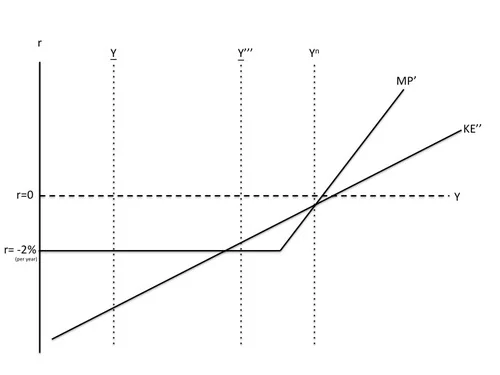
But a still bigger increase in government purchases combined with a zero nominal rate up to an even higher level of output might do the trick, as shown below.
“Stagnation”
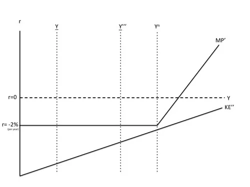
Of course, there is the logical possibility that the risk-adjusted net rental rate might be below -2% per year even at the natural level of output. In this situation, the zero lower bound makes it impossible to reignite generic investment (until longer-run forces intervene, such as the gradually wearing away of the generic capital stock).
How Eliminating the Zero Lower Bound Deals with Stagnation
Even the stagnation situation is compatible with getting back to the natural level of output if the zero lower bound has been eliminated. The real interest rate would be below -2% at the natural level of output, reflecting some combination of bad supply-side factors, but monetary policy would be handling those supply-side factors as gracefully as possible.